

The samples investigated in this work are based on the design of a purely two-dimensional stealthy hyperuniform disordered dielectric network, shown in Fig. 1a, generated using the tessellation protocol described in ref. 10 (see “Materials and methods” section for details). Stealthy hyperuniform structures37,38 are disordered point patterns whose structure factor vanishes exactly within a finite region of reciprocal space, i.e., \(S\left({\bf{k}}\right)=0\) for \({\rm{| }}{\bf{k}}{\rm{| }} < {k}_{{\rm{C}}}\), where kC is a cutoff wavenumber. The stealthiness parameter χ quantifies the fraction of constrained wavevectors and controls the strength of long-range correlations. In the large-χ limit, stealthy hyperuniform patterns approach crystalline order, whereas small χ corresponds to reduced structural constraints, and hence more disordered, hyperuniform structures8,10. Analogously to the lattice constant in photonic crystals, a length scale \(a=L/\sqrt{N}\) is defined, such that an N-point hyperuniform pattern in a square box of side length L has a scatterer density of \(1/{a}^{2}\) (here we use the stealthiness parameter χ = 0.510, N = 4000, and a = 380 nm). The photonic band structure of the sample for transverse-electric (TE) polarization is calculated using a supercell approach, exploiting the fact that the HuD pattern is generated under periodic boundary conditions, and is shown in the left panel of Fig. 1b. The resulting band structure exhibits a photonic band gap of approximately 23% of its central frequency.
Fig. 1: HuD network design, photonic band structure and energy-level statistics. The alternative text for this image may have been generated using AI.
a Sketch of the 24 × 24 μm2 2D theoretical design of the HuD network with N = 4000, length scale a = 380 nm, wall thickness u = 0.34a and stealthiness χ = 0.5. b Left panel: 2D photonic band structure, with a/λ is the dimensionless frequency, and the high-symmetry directions in the reciprocal space defined by the irreducible Brillouin zone of the hyperuniform disordered sample. Right panel: localization length ξ of the HuD structure as a function of frequency, with the photonic band gap region of the corresponding honeycomb periodic structure (at the same filling fraction) highlighted as a dotted area. The spectral regions for which the level statistics are best fit by the Poisson distribution are shaded in light orange, while the ones for which the level statistics are best fit by the Wigner–Dyson distribution are shaded in light blue. The plot displays the calculated localization length for 50 samples and 17 k-points per sample (in black). The red curve represents a spline fit of the average value \(\langle \xi /a\rangle\) in a narrow frequency range Δ[a/λ] = 5 × 10⁻³ around the frequency a/λ considered. The white region in the middle refers, accordingly with the left panel of (b), to the photonic band gap of the HuD pattern for χ = 0.5. c Level-spacing distribution for modes with frequencies in the lower blue region of the right panel of (b) and corresponding Wigner–Dyson distribution. d Level-spacing distribution for modes with frequencies in the lower orange region of the right (b) and corresponding Poisson distribution
It has been previously demonstrated that the interplay of hyperuniformity, short-range geometric order, and uniform local topology results in the formation of a complete PBG10; its formation is directly linked to the Mie-like resonances10,39,40,41 of the individual scattering centers (for transverse magnetic, TM, polarization) or scattering cells (TE polarization) within the structure, when the scattered field is out of phase with the incident field, resulting in the absence of propagation channels for light42. Firstly, we numerically characterize the localization properties of the modes through the average localization length ξ (defined as in ref. 24 by ξ = (1/2)\(\sqrt{1/{IPR}}\) with \({IPR}\) the Inverse Participation Ratio) at different frequencies, obtained by evaluating the average intensity distributions of 50 different realizations. Due to the size of the computational problem, we limit the localization length analysis to smaller samples consisting of 500 points each. The right panel of Fig. 1b reports the localization length ξ of the HuD structure as a function of frequency, with the photonic band gap region of the corresponding honeycomb periodic structure (at the same filling fraction) highlighted by the dotted area. This plot confirms that in HuD structures, low-frequency modes below the band gap have extended spatial profiles (larger ξ) that indicate a diffusive regime, while at higher frequencies closer to the photonic band edges, the modes become much more localized (smaller ξ)16.
A central challenge in disordered photonics is distinguishing between localized and delocalized states, i.e., establishing a quantitative measure to reliably classify optical modes according to their spatial extent. Spectral level repulsion is a universal signature of modal overlap20,21,22,23,27: the link between modes spatial localization and their eigenfrequency is at the basis of the level repulsion phenomenon, as it is directly related to the spatial extension of the photonic modes present in the structure; for modes whose spatial extent covers a large fraction of the sample, overlap is unavoidable and in order to maintain orthogonality the modes “repel” each other in the frequency domain and hence need to have different frequencies24. We therefore approach the distinction between localized and delocalized modes with numerical simulations in 2D through the level-spacing statistics method24,25,27. Defining \({s}_{n,k}=\frac{\Delta {\omega }_{n}(k)}{\left\langle \Delta {\omega }_{n}(k)\right\rangle }\) as the dimensionless spacing between adjacent bands n and n + 1, with \({\mathrm{\varDelta \omega }}_{n}\left(k\right)={\omega }_{n+1}\left(k\right)-{{\rm{\omega }}}_{n}(k)\), the delocalized mode spacings are characterized by the Wigner–Dyson distribution24,28
$$P\left(s\right)=\frac{{\rm{\pi }}s}{2}\,exp\left(-\frac{{\rm{\pi }}{s}^{2}}{4}\right)$$
(1)
for which \(\mathop{lim}\limits_{s\to 0}P\left(s\right)\to 0\). In contrast, localized modes with field distribution confined to disjoint regions of the sample are spectrally uncorrelated. The mode’s level statistics are therefore characterized by a Poisson distribution,
$$P\left(s\right)=exp\left(-s\right)$$
(2)
and the modes can have arbitrarily close frequencies since the level repulsion is absent: \(\mathop{lim}\limits_{s\to 0}P\left(s\right) > 0\). To identify the spectral ranges over which the level-spacing statistics are best described by either a Poisson distribution or a Wigner–Dyson distribution, we perform a global search for chi-square minimization of the respective distributions. We find that regions located at the band-edge for \(a/{\lambda }\in \left(0.221,\,0.236\right)\cup \left(0.284,\,0.304\right)\) (highlighted in light orange in the right panel of Fig. 1b), the level spacing is best described by a Poisson distribution (see Fig. 1d), whereas for \(a/{\lambda }\in \left(0.041,\,0.221\right)\cup \left(0.304,\,0.353\right)\) (highlighted in light blue in the right panel of Fig. 1b), the level statistics is best described by the Wigner–Dyson distribution (see Fig. 1c). We note that the level-spacing analysis is performed over finite frequency intervals, whose boundaries are systematically varied to identify the ranges best described by Wigner–Dyson or Poisson statistics. As a result, the assigned statistics represent dominant spectral regimes rather than individual modes, and Wigner–Dyson behavior may persist even when the average localization length within an interval remains only a few times the characteristic length scale a.
Interestingly, the Wigner–Dyson level-spacing statistics observed for delocalized modes correspond to the Gaussian Orthogonal Ensemble (GOE) of random matrix theory, the appropriate universality class for time-reversal-symmetric wave systems (see, e.g., ref. 28). Beyond the familiar level repulsion behavior at small spacings, GOE spectra exhibit pronounced spectral rigidity, whereby fluctuations in the number of levels within large frequency intervals are strongly suppressed relative to uncorrelated (Poisson) sequences. In the language of point processes, this suppression of long-wavelength spectral fluctuations is the spectral analog of hyperuniformity: GOE eigenvalue sequences are themselves hyperuniform in one dimension8. This correspondence points to a close connection between the structural correlations of stealthy hyperuniform media and the long-range correlations emerging in their mode spectra. At the same time, real-space hyperuniformity alone does not imply GOE statistics; rather, GOE-like behavior arises from significant modal overlap and interaction, consistent with the delocalized transport regime identified here.
We experimentally investigate these two regimes in HuD structures by exploiting the subwavelength resolution of SNOM to resolve the spectral and spatial structure of delocalized modes of samples realized with the optically active slab technology12,16,17: a 8 × 8 μm2 crop of the HuD pattern (highlighted by the red rectangle in Fig. 1a) was employed to pattern a GaAs 220-nm-thick membrane with InAs quantum dots embedded in the middle. More details on the sample fabrication and SNOM technique can be found in the “Materials and methods” section. In the following, we focus on dielectric modes below the PBG and across the lower band-edge. In Fig. 2a it is reported a typical SNOM PL spectrum acquired at a fixed position on the structure, whose details can be observed in the Scanning Electron Microscopy (SEM) image (top panel of Fig. 2b). The spectrum exhibits a high density of peaks of different intensity and spectral width, corresponding to different light transport regimes16, coherently with the theoretical results shown in Fig. 1: after the PBG region, dielectric localized modes with sharp peaks and high-quality factors arise (light orange area). Farther from the PBG edges, broader resonances with delocalized spatial distributions appear, indicating a diffusive regime (light blue area). The hyperspectral SNOM Photoluminescence (PL) map filtered around the entire spectral window ∆λ = [1175–1290] nm allows to clearly visualize the collective spatial distributions of the dielectric modes at the PBG lower edge (Fig. 2b lower panel). Since the contribution of level repulsion to macroscopic spectra is very weak, if not absent, we leverage the spatially resolved SNOM technique, which selectively excites only modes close to each other in real space, enabling a direct insight into this universal signature of mode spatial overlap. Moreover, given the finite dimension of the sample and therefore the limited number of modes supported by the physical structure, to experimentally detect the level repulsion phenomenon, we do not rely on the level-spacing statistics approach24 that requires a large number of modes to guarantee reliable results. Instead, we evaluate the autocorrelation function of the experimental near-field spectra, which is expected to be strongly influenced by level repulsion features for small spectral separations (∆λ)22,26. Indeed, the autocorrelation function Rc (∆λ) represents a microscopic statistical property of the system and can be evaluated by averaging the autocorrelation of the single spectra collected in every pixel of the SNOM hyperspectral map (Fig. 2b bottom panel) and subtracting the uncorrelated contribution given by the autocorrelation of the average of all the spectra in the map. The full procedure is described in refs. 22,26 and summarized in Section S1 of the Supplementary Information. The autocorrelation function constitutes a different observable from the nearest-neighbor spacing distribution: for Wigner–Dyson statistics, level repulsion implies that the two-level correlation function vanishes at zero separation. In an idealized system of infinitely sharp spectral lines, this would manifest as a suppression of correlations, \({R}_{c}\to 0\), as \(\Delta \lambda \to 0\), corresponding to a dip in the autocorrelation function at small spectral separations. In practice, each discrete energy level has a finite Lorentzian linewidth, and the self-correlation of these Lorentzians generates a pronounced peak in \(R(\Delta \lambda )\) at \(\Delta \lambda =0\), as shown in previous studies22,26. As a result, when reconstructing \({R}_{c}(\Delta \lambda )\) experimentally, the ideal dip associated with level repulsion does not appear as a zero at \(\Delta \lambda =0\), but instead emerges as a characteristic shoulder or minimum at a finite Δλ. The position of this feature is determined by the interplay between the mean level spacing and the Lorentzian linewidth. By contrast, for spectra obeying Poisson statistics, where level repulsion is absent, \({R}_{c}(\Delta \lambda )\) does not exhibit such short-range suppression and is dominated solely by the central peak.
Fig. 2: Experimental observation of spectral level repulsion through SNOM hyperspectral imaging.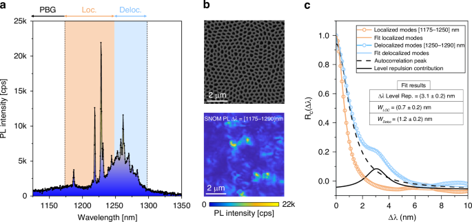 The alternative text for this image may have been generated using AI.
a Typical SNOM PL Intensity spectrum acquired in a single position of the tip on the HuD sample; the spectrum is divided into three regions, highlighting the PBG, the localized modes, and the delocalized modes. b Upper panel: SEM image of a detail of the patterned membrane. Bottom panel: SNOM PL collective map filtered around the spectral window (1175–1290 nm) displaying the spatial distribution of Anderson resonances on the sample. c Autocorrelation function Rc (∆λ) evaluated in the spectral windows corresponding to the localization (light orange curve, (1175–1250 nm)) and delocalization regimes (light blue curve, (1250–1290 nm)). The sampling over ∆λ is 0.11 nm, corresponding to the spectral resolution of the setup. The two curves are fitted respectively with a Lorentzian (orange) and a sum of two Lorentzian peaks (blue)
In our sample, \({R}_{c}(\Delta \lambda )\) must be evaluated in two different spectral windows, given the different localization length of the modes sustained by the sample. In Fig. 2c we report the two curves of \({R}_{c}(\Delta \lambda )\) calculated within the localized modes spectral window (1175–1250 nm) (light orange curve) and delocalized modes (1250–1290 nm) (light blue curve). For more details on the data processing methods and criteria of choice of spectral intervals, see Section S1 of Supplementary Information. For both cases, we observe the autocorrelation peak that occurs for the self-correlation of each spectrum (∆λ = 0 nm). This broadened peak weakens the level repulsion dip into a shoulder, clear in the light blue curve and centered at ∆λ = (3.1 ± 0.2) nm as extracted by the fit. In contrast, the autocorrelation of localized modes does not exhibit any trace of level repulsion, proving that they are uncorrelated. Interestingly, our technique provides an additional physical insight into the photonic features of modes. The autocorrelation peak is narrower for localized modes characterized by higher quality factors, Q, than the delocalized ones (Q is defined as the ratio between the resonance wavelength and its linewidth, \(Q={\lambda }_{0}/w\), and hence quantifying the lifetime of an optical mode). It can indeed be used to indirectly measure the typical spectral width of the modes in the two regimes; the values extracted from the fits result in wLoc = (0.7 ± 0.2) nm and wDeloc = (1.2 ± 0.2) nm, in excellent agreement with the previously reported Q-factor theoretical results16. To get a better comparison with 2D theoretical simulations (Fig. 1), taking into account the scaling factor necessary to convert between the frequencies of the 2D structure and the 3D slab one (~1.32516), we obtain that the experimental spectral limit among the two ranges (1250 nm) is in normalized frequency values a/λ = 0.229, in almost a perfect agreement with the numerical simulations (a/λ~0.221). Residual deviations between theoretical and experimental spectral measurements must be attributed to a variation in the filling fraction introduced by the fabrication process and slight modifications in the slab thickness.
Having reliably distinguished between delocalized and localized modes, we now focus on the latter. As in other disordered systems24, two distinct types of localized states can occur in hyperuniform disordered networks10,12,16: (i) genuine Anderson-localized modes, which arise from strong disorder and multiple scattering throughout the structure and are not strictly confined to band-edge regions. These resonances reflect a disorder-driven transition from extended to localized states and are associated with Wigner–Dyson and Poisson statistics for delocalized and localized modes, respectively, as indicated by the light blue and orange regions in the left panel of Fig. 1b. (ii) defect-induced, tightly localized modes, which are confined to only a few cells10,12,16 and are spectrally located in the immediate vicinity of the band edges. These modes are promoted into the band gap of the corresponding periodic structure by the presence of hyperuniform disorder.
The two types of localized modes can be distinguished by analyzing their localization length at different degrees of disorder. In the HuD system, smaller values of the stealthiness parameter χ correspond to a higher amount of disorder10. By analyzing the localization length of HuD modes as a function of χ, we can discriminate between genuine Anderson-localized modes, whose localization length decreases with increasing disorder, and defect-induced modes, with localization length increasing with the degree of disorder present in the sample10,24. The results of this calculation, employed here as an operational and platform-specific method, are shown in Fig. 3a, where the ξ of the HuD structure is reported as a function of frequency for values of χ varying from 0 to 0.5 (more simulation results can be found in Supplementary Information, Fig. S2.1, showing ξ vs frequency for three sample sizes). The colors in the spectral windows are overlapped accordingly with the ranges investigated in Fig. 1. We observe that all ξ curves on the left side of Fig. 3a cross within a narrow spectral region centered around a/λ = 0.227, precisely defined by the lower PBG edge of the honeycomb periodic structure of the same filling fraction (highlighted as a dotted pattern in the figure). This coincidence is not arbitrary: in this frequency window, disorder no longer simply perturbs extended dielectric-band modes into Anderson-localized modes but starts promoting tightly localized resonances into the band gap. This is a first clue suggesting a transition from type (i) to type (ii). In the \(a/{\lambda }\in\) (0.221–0.227) spectral range (highlighted in light orange), the modes can be labeled Anderson-localized (type (i)) as their ξ decreases a χ decreases (details on fluctuations and extra spectral range can be found in Supplementary Information, Fig. S2.2). We note that the nature of the Anderson modes above the upper band-edge of the photonic band gap of the HuD structure is rather distinct from that of the photonic modes below the lower band-edge. This difference is a quintessential of the HuD architecture employed here. Modes below the photonic band gap, the so-called “dielectric band”, have the electric field mostly concentrated in the dielectric fraction of the structure. Since the dielectric is structured as a connected network with walls of constant thickness and uniform trivalent connectivity, for the “dielectric-band” modes, the disorder manifests itself only as fluctuations in the coupling between electromagnetic resonances set up in the spatially uniform distribution of dielectric material. We note that the effect of the disorder is hence limited, and it results in a relatively small shift of the lower band gap edge compared to the periodic counterpart structure (a perfect honeycomb network of the same filling fraction). In sharp contrast, the photonic modes above the band gap, the so-called “air-band”, have most of the electric field concentrated in the air fraction of the HuD structure, i.e., inside the cells of the HuD network. While the dielectric fraction suffers only from positioning disorder, the air fraction of the network is subject to two concomitant hyperuniform disorder effects. On one hand, similarly to the dielectric fraction, the distance between the “air” cells varies across the sample (positional disorder), and, on the other hand, the cells have now different sizes and shapes (“form” disorder). This combined position, shape, and size disorder has a major influence on the upper band-edge modes, and as shown on the right panel of Fig. 1b, a much larger number of them are promoted inside the band gap of the corresponding periodic honeycomb structure.
Fig. 3: Disorder-dependent localization crossover and emergence of Lifshitz-like defect states in HuD photonic networks. The alternative text for this image may have been generated using AI.
a Localization length ξ of the HuD structure for different values of the stealthiness parameter χ, as a function of frequency. The white region in the center denotes the true photonic band gap of the hyperuniform disordered pattern at χ = 0.5, the value considered in this work, analogous to the right panel of Fig. 1b. This gap defines the spectral region associated with the orange and blue areas, corresponding to Poisson and Wigner–Dyson statistics. Upon decreasing χ, the band gap progressively shrinks and closes at χ = 0.2. The overlaid dotted pattern marks the gap of the corresponding periodic structure of the same filling fraction. b Histogram of four-sided topological defects (sketched in the inset) in different realizations of HuD networks varying N (500, 1000, 10,000, and 30,000) and for increasing values of χ, corresponding to decreasing degree of disorder
For frequency above a/λ = 0.227, defect modes (type (ii)) of a special kind are being formed, with ξ increasing for smaller values of χ. These defects in HuD platforms come with a peculiar cavity-like feature due to their association with topological defect modes hosted by four-sided cells in the honeycomb-like hyperuniform network10,12,16 (see inset in Fig. 3b). With reference to the photonic band structure (left panel of Fig. 1b), the miniband inside the PBG consists of 12 defect modes matching precisely the number of four-sided-cell defects (highlighted in red in Fig. 1a) present in the structure. Four-sided cells modes are indeed invariably promoted inside the PBG of the correspondingly periodic honeycomb structure (corresponding to a frequency range \(a/{\lambda }\in\) (0.227–0.349) and highlighted by the dotted area in Fig. 1b, right panel), displaying the tightest spatial localization of all the modes (Fig. 3a)12. Beyond the trend of ξ, the spectral and spatial peculiarities of four-sided-cells defects demonstrate that the introduction of a controlled amount of hyperuniform disorder (by changing χ) leads to a smooth crossing, occurring at the lower edge of the corresponding periodic honeycomb structure’s PBG, between modes of different nature. An additional analysis based on the band structure and mode profiles at the crossover in the localization behavior is reported in Supplementary Information, Fig. S3.1.
We argue that the modes associated with four-sided cells, which form a miniband within the photonic band gap, can be interpreted as the photonic analog of Lifshitz states known from electronic systems. In a hyperuniform disordered architecture, their peculiar topological origin implies a degree of predictability in their spatial location. To demonstrate this, we evaluate the occurrence of these states in the HuD sample of different sizes (N = 500, 1000, 10,000, and 30,000 points) for increasing values of χ (i.e., decreasing degree of disorder). The results, reported in Fig. 3b, show with extreme clarity that the number of four-sided-cell defects not only increases with the sample size (N), but also with disorder. In the strict statistical-mechanical sense, Lifshitz states are defined as exponentially rare, disorder-induced eigenmodes whose occurrence governs the asymptotic behavior of the density of states near a band-edge, giving rise to Lifshitz tails in the thermodynamic limit29,30,31,32. Demonstrating such states rigorously requires large-scale statistical simulations of the density of states over many disorder realizations and system sizes, as recently discussed for hyperuniform systems in ref. 32 While such an asymptotic analysis is beyond the computational scope of the present work, the localized band-edge modes observed here display the key phenomenological hallmarks commonly associated with Lifshitz physics: strongest spatial confinement, spectral proximity to the band-edge, and a disorder-induced origin (for a more detailed analysis of how the concentration of these states varies with sample size, see Fig. S3.2 of the Supplementary Information). Here and in the following, these states are referred to as “Lifshitz-like” states.
In this scenario, one consequence of increasing the degree of disorder is that, due to their increased concentration, Lifshitz-like states localization is degraded, and weak spatial overlap can enable hopping-like transport, analogous to Mott’s variable-range hopping in electronic systems43. We therefore focus on the five Lifshitz-like states present in the fabricated samples, mapping their near-field spatial distribution with the hyperspectral PL map (filtered around ∆λ = [1150–1220] nm) reported in Fig. 4a. A pair of two spatially near Lifshitz-like defects can be spotted among the five modes (yellow rectangle in Fig. 4a).
Fig. 4: Hybridization of Lifshitz-like states into a photonic molecule. The alternative text for this image may have been generated using AI.
a SNOM PL map filtered around the PBG region where five Lifshitz-like states can be visualized. b SNOM PL spectra, each acquired on top of a single four-sided cell defect, and relative Lorentzian fits. The points of acquisition are highlighted by the orange triangle and purple square in the corresponding spectral shift maps, shown in (c). d FEM maps of the electric field intensity of the coupled Lifshitz-like defects. e Corresponding FEM maps of the out-of-plane magnetic field (Hz), revealing bonding and antibonding behavior with locally symmetric and antisymmetric field distributions, respectively
We measure the local electric field intensity by evaluating, through Lorentzian fits, the tip-induced spectral shift12 on the two corresponding modes. Figure 4b reports the fitted PL spectra acquired in two different positions of the hyperspectral map, each corresponding to one of the two individual defects; we observe that the two peaks representing the two modes can be found with different weights on both defects. The morphological information given by the SNOM topography (see Supplementary Information, Fig. S3.3), combined with the spectral shift maps reconstructed by fitting the spectra in each pixel, allows us to establish that the signal of the two modes (Fig. 4c) is delocalized on both Lifshitz-like states. The spatial delocalization, together with the spectral splitting of ∆ = 11.4 nm, indicates a coupling between the two modes. We validate this observation through Finite-Element Method (FEM) simulations, whose maps of the electric field intensity are reported in Fig. 4d: despite the rigid spectral shift between theory and experiment (to be attributed to discrepancy between nominal and fabricated structural parameters like slab thickness and filling fraction) the FEM maps are in excellent agreement with the SNOM maps and the theoretical spectral splitting of ∆ = 9.6 nm is comparable with the experimental one. Moreover, Fig. 4e illustrates, through Finite-Element Method maps of the transverse magnetic field component (Hz), the bonding and antibonding behavior characteristic of photonic molecules. To our knowledge, there is no prior experimental observation in electronic systems of hybridized Lifshitz tail states forming resolvable bonding–antibonding pairs. While theory predicts hybridization/splitting of localized levels in Lifshitz-type models44 and classic impurity-band studies imply overlap among tail states as concentration increases45, a direct experimental demonstration has never been accomplished. In photonic systems, previous studies of uncorrelated random media have reported hybridization only through local tuning or perturbative modifications8,36. Our results instead indicate that hyperuniform structures, while disordered, support an architecture-encoded predictability that enables controlled hybridization without post-fabrication tuning. This finding is extremely important since, when several of such localized states align spatially and spectrally, they can hybridize to form optical necklace states3,7,35,36, which act as cooperative pathways for light propagation through the disordered structure. Thus, photonic Lifshitz-like states serve as the building blocks for more complex phenomena, from photonic dimers to full necklace states, mediating sub-gap transmission in disordered photonic media. Our results thus provide the first clear evidence of this phenomenon and, given the special architecture upon which they rise in HuD, the aspect of predictability is then brought into the picture of these rare statistical events, making our findings unique and impactful.