
Bayesian Hierarchical Modeling with BAYEX
The BAYEX framework4 performs spatiotemporal Bayesian hierarchical modeling of coastal storm surge extremes and is represented as a product of conditional distributions or sub-models, or layers. These comprise: (1) an “observation model” that links the prescribed extreme data to the spatio-temporal processes; (2) a “process model” that accounts for underlying dynamics of the processes involved; and (3) a “parameter model” that considers the underlying uncertainties in the parameters and integrates any prior knowledge about the prescribed data and underlying processes. The hierarchical model structure enables the assessment of the joint distribution of the processes and parameters conditioned on the data (also known as the posterior distribution), while rigorously propagating the uncertainties underlying the data, processes, and parameters4. These types of Bayesian Hierarchical Models (BMH) have been applied across various science disciplines (e.g., hydrology20 and ecology21) to enable robust statistical estimates, especially in contexts characterized by data scarcity and high uncertainty.
In modeling spatial inter-site dependences of storm surge extremes, BAYEX resolves residual dependence (sites with co-occurrence of storm extremes) and climatological dependence (sites with similar and/or consistent storminess but not necessarily co-occurrence of storm extremes). Residual dependence is resolved using a max-stable process4,16,22 (i.e., an infinite-dimensional generalization of a Generalized Extreme Value (GEV) distribution) and storm climatological dependence is here captured using latent Gaussian processes with random effects and physical bathymetric covariates (continental shelf width estimated using Natural Earth 200-meter depth contour line)4. In other words, residual dependence implies dependence among annual maxima whereas climatological dependence reflects spatial association amongst the GEV parameters4. The marginal distribution at any particular site follows a univariate GEV distribution based on max-stable process theory, with parameters μ (location), σ (scale), and ξ (shape). The location parameter, μ, is modelled as a spatial time-evolving process (using an integrated random walk) to account for climatological storm frequency changes. The GEV scale and shape parameters follow a spatial-varying, stationary process. An extensive description of BAYEX including its formulation, implementation and testing, has already been provided elsewhere4,14, and thus we only provide a brief description of its observation and process model layers. The likelihood can be written as4,22:
$${Y}_{t}\left({s}_{i}\right)|{\theta }_{t}\left({s}_{i}\right),{\mu }_{t}\left({s}_{i}\right),\sigma \left({s}_{i}\right),\xi ({s}_{i}),\alpha \sim {GEV}\left({\mu }_{t}^{* }\left({s}_{i}\right),{\sigma }_{t}^{* }\left({s}_{i}\right),\alpha {\xi }^{* }({s}_{i})\right),$$
(1)
$${\mu }_{t}^{* }\left(s\right)={\mu }_{t}\left(s\right)+\frac{\sigma (s)}{\xi }\left({{\theta }_{t}\left(s\right)}^{\xi (s)}-1\right),$$
(2)
$${\sigma }_{t}^{* }\left({s}_{i}\right)=\alpha \sigma \left(s\right){{\theta }_{t}\left(s\right)}^{\xi \left(s\right)},$$
(3)
where \({Y}_{t}\left({s}_{i}\right)\) is the annual maximum surge (m) for year \(t\) at site \({s}_{i}\), and \({\theta }_{t}\left(s\right)\) is a spatial process resolving residual dependence and \(\alpha \) ∈ (0,1) is a parameter that controls the relative contribution of small-scale errors. The GEV shape parameter, ξ, is allowed to vary in space, according to a Gaussian process18:
$$\xi (s) \sim GP(\underline{\xi },c(s,s{\prime} ;{\gamma }_{\xi },{\rho }_{\xi })),$$
(4)
where \(GP(\underline{\xi },c(s,s{\prime} ;{\gamma }_{\xi },{\rho }_{\xi }))\) is a Gaussian process with mean \(\underline{\xi }\) and covariance function c(,∙). The hyperparameters \({\gamma }_{\xi }\) and \({\rho }_{\xi }\) denote, respectively, standard deviation and length scale values defining the covariance function4.
The GEV location parameter \({\mu }_{t}\left(s\right)\) is assumed to vary smoothly through time (to resolve long-term changes such as nonlinear trends as opposed to shorter-term variations, which are likely unresolvable) using a spatio-temporal integrated random walk according to4:
$${\mu }_{t}\left(s\right)={\mu }_{t-1}\left(s\right)+{\mu }_{{trend},t-1}\left(s\right),$$
(5)
$${\mu }_{{trend},t}\left(s\right)={\mu }_{{trend},t-1}\left(s\right)+{\omega }_{t}\left(s\right),$$
(6)
where \({\omega }_{t}\left(s\right)\) is a zero-mean Gaussian process \({\omega }_{t}\left(s\right) \sim {GP}\left(0,c\left(s,s{\prime} ;{\gamma }_{\mu },{\rho }_{\mu }\right)\right)\).
The extended description of all BAYEX process layers and parameters, including all Gaussian processes and initial states of \(\mu \), see refs. 4,5. The full description of the BAYEX spatial domain and the statistical inference process and model diagnostics analysis has been provided in ref. 18. In total, 6,000 distribution samples (post-warm-up draws for analysis) are provided by BAYEX (after a warm-up phase) for gauged and ungauged sites along the U.S. coastline (Fig. S1)18.
Observational data for BAYEX
US-CoastEX includes extreme skew surge distributions (Fig. S3 shows posterior-median and 90% credible intervals) in addition to ESL estimates derived through BAYEX based on annual maximum skew surge data obtained from different data sources (Tables S1–S2) as shown below and illustrated in Fig. 1.
Fig. 1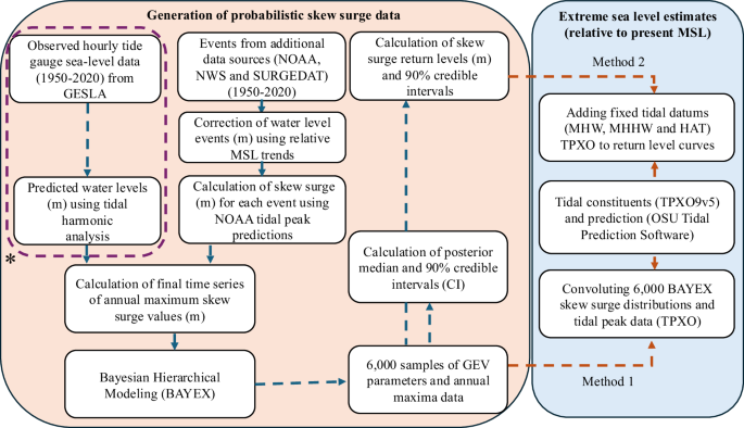
Methodological framework diagram. The orange-shaded section displays the general workflow used to generate BAYESL-TG/EXT while the blue-shaded section shows the general workflow used to estimate the extreme sea level data from BAYESL-TG/EXT. The application of BAYES-TG uses only annual maxima skew surge data from observed hourly tide gauge sea-level records (as shown by the dashed violet line and the asterisk ‘*’).
Standard version (BAYESL-TG)
In the standard application of BAYEX (henceforth BAYESL-TG), the model is informed solely by historical time series of annual maxima skew surge (used synonymously with storm surge) derived from high quality hourly sea-level records (1950–2020) from 208 open-coast tide gauge sites included in the GESLA-2 (Global Extreme Sea Level Analysis) database (retrieved from: https://www.bodc.ac.uk/resources/inventories/edmed/report/6562/)23 (Figs. S1, S2). Skew surge (defined as the absolute difference between observed high-water level and the closest predicted high tide regardless of their timing over a tidal cycle) has been shown to be a reliable metric of storm surge under different tidal regimes24. Note that tide gauge data included in GESLA-2 are very similar to records in GESLA-3, as most updates and new data are for estuarine, river and lake regions, which are not used here, as further discussed below. We require 70% of all hourly records over a given year to determine an annual maximum. We remove any underlying mean sea level changes and its underlying variability by removing a centered 30-day moving average from the observed water level data. The data is also visually scrutinized and the corrected when required for any datum shifts and tsunamis. The tidal signal was extracted using a year-by-year harmonic analysis. This analysis is entirely focused on open-coastal regions where storm surge extremes are mainly driven by wind and pressure effects. Therefore, only tide gauges within a maximum of 5 km from a coastline are used and locations further within deltas, narrow inlets, bays and tidal rivers, have been removed to minimize major effects of hyper-local geography, river discharge and/or nonlinear interactions which generally lead to very different storm surge extremes than events experienced along open-coastal regions. The full description of the data processing is available elsewhere18. The exact location of the tide gauge sites, and their record length, are shown in Fig. S1. The samples of GEV model parameters (summarized as posterior-medians and 90% CI within Fig. S3) and annual maxima from BAYESL-TG/EXT are archived without further processing (Table S3). A full discussion of BAYESL-TG extreme skew surge data is also provided in ref. 18.
Extended version (BAYS-TG/EXT)
Hourly tide gauge records provide high-quality ESL information but since they generally have hourly resolution, they could miss absolute peaks of storm events when there are larger changes in water levels at sub-hourly levels, as occurs more often during major events. In addition, it is well documented that during major storms (e.g., Camille and Katrina) there is typically missing data due to tide gauge damage or malfunction25,26. Hence, we provide an extended-data version (BAYESL-TG/Extended) where BAYEX has been informed not only by historical time series of annual maxima skew surge from hourly sea-level records, but also with extreme surges from NOAA top-ten water level data archives (https://api.tidesandcurrents.noaa.gov/dpapi/prod/)27, including 6-min tide gauge records (after 1996), inferred extremes (derived through gap-filling procedures due to missing data), last recorded extreme water levels (last successfully recorded level before tide gauge malfunction during a storm) and high water marks and storm-tide peaks from SURGEDAT’s database (https://surge.climate.lsu.edu/data.html#GlobalMap) (Tables S1–S2)26. In Fig. 1 (and Table S1 and Fig. S4) we present a brief comparison of BAYESL-TG and BAYESL-TG/EXT. The top-ten water-level information data from NOAA contains tide gauge codes, station names, peak dates & times, height, datum (MSL) and source27. The SURGEDAT data26 provides location, year and datum (for specific events) and recorded (or observed) water level data. Storm surge events before 1950 and after 2020 have been removed for consistency. Storm events retrieved from SURGEDAT26 are only considered when reported as ‘storm tides’ (without breaking wind-wave influence) and with datum (described as height relative to normal tides, i.e., MSL) and their documented locations are within 20 miles from a tide gauge. The peak date and time are retrieved from NOAA’s extreme water level meteorological reports and confirmed using historical hurricane track data28. Any extreme events prior to 2020 have been updated (or corrected) to present-day MSL (2020) by adding MSL rise between the year of the recorded events and 2020) using relative MSL trends estimated by NOAA. There are a few tide gauge locations where no relative MSL trends are available and thus the values from the nearest tide gauge locations are used. The skew surge associated with each extreme water level event is determined by removing the closest tidal peak values extracted from NOAA’s tide prediction records, using their respective peak date and time, with all events brought to the same reference datum (MSL). For events where peak times are not provided (or available), tidal peak averages from that particular day have been used. In total, 1084 skew surge events have been estimated. We then compare these values with annual maxima skew surges previously estimated for those years using hourly tide gauge data, i.e., used to inform BAYESL-TG as previously described. The highest values within each year are therefore used as annual maxima. In total, 775 annual maxima skew surge values estimated from hourly tide gauge data are replaced by new, updated annual maxima skew surges, 652 obtained from processed NOAA top-ten water-level data, 2 from NOAA NWS data archives, and 7 from the SURGEDAT (Table S2). BAYESL-TG/EXT (extended version) and BAYESL-TG (standard version) use the same values for Alaska, Puerto Rico and the U.S. Virgin Islands, since no relevant annual maxima events have been identified across other complementary data sources (i.e., compared against annual maxima obtained from standard hourly tide gauge records). The GEV parameters associated with BAYESL-TG and BAYESL-TG/EXT are archived without further processing (see Table S3).
Estimation of ESL return levels using BAYEX outputs
ESL occurrences depend upon tidal processes and storm surges29. Here we use two approaches that are typically used to calculate ESL return levels from skew surge and tidal data29. The first approach (henceforth “Method 1”) convolves the probability distributions of deterministic tidal peak data and stochastic storm surge data. This convolution approach allows us to use complete tidal information, which is not possible through direct analysis of still water levels (Fig. S5)29. The probability of a given ESL event is thereafter derived from the joint cumulative distribution function. The convolution integral is given by29:
$$F\left(z\right)=\int {G}_{r}\left(z-x\right)f\left(x\right){dx}$$
(7)
where \({G}_{r}\) is the (GEV) distribution of extreme skew surges and \(f\) is the density function of the tidal peaks over a full 18.61-year nodal tidal cycle. This approach assumes skew surge and tide independence with an equal probability of a given skew surge occurring at any high tide28. We convolve 6,000 skew surge distribution samples from BAYEX with tidal peak data, generating a total of 6,000 ESL return period curves from which posterior-median values and associated 90% credible intervals are calculated. The second approach (henceforth Method 2) adds a fixed tide level (such as Mean High Water (MHW), Mean Higher High Water (MHHW), or Highest Astronomical Tide (HAT)) (Fig. S6) to estimates of extreme surge levels9,23. Although we use Method 1 as reference in this analysis, we also provide alternative ESL estimates derived using fixed tide levels MHW, MHHW, and HAT (Fig. S6), aligning with previous research15,29; but other tidal levels could be used. The observed tidal peaks at gauged locations are obtained from GESLA water level time series via harmonic analysis (using the same time series from which annual maxima skew surge levels are obtained to inform BAYEX). Fig. S5 shows a comparison of 100-year ESL events derived using the different alternative methods at tide gauge sites using GESLA-based tidal peak data. The comparison shows that Method 1 (convolution) and Method 2 (when adding MHHW to estimates of storm surge return levels) result in consistent 100-year ESL return levels almost everywhere (differences of less than 0.20 cm); except along macro-tidal coastal regions where tidal influences dominate over maximum surge levels (e.g., Gulf of Alaska and/or Bay of Fundy). The 100-year ESL return levels obtained using HAT (Method 2) illustrate a very conservative (assume that extreme surge events always happen during HAT29) and exceed estimates from Method 1, everywhere, particularly on coastlines with considerable tidal ranges as mentioned before.
At ungauged sites, high tide values are derived by applying harmonic analysis to the barotropic tidal TPXO9-atlas model (version 5) dataset, a product that exhibits a very small deviation (<10 cm) in terms of harmonic constituents relative to tide gauge data (https://www.tpxo.net/home)30,31. The distribution of high tides from TPXO9v4 spans a full 18.6-year nodal tidal cycle. The comparison of MHHW and HAT tide levels from TXPO9v5 and GESLA for tide gauge stations (Fig. S6) shows that TPXO9v5 and GESLA-based MHHW and HAT agree well at most coastal sites with absolute differences of less than 0.1 m and 0.3 m, respectively. Note that tidal peak records from other tidal model products could be used to determine ESL estimates at ungauged sites based on BAYEX skew surge data. Figure 2 presents 100-year ESL return levels (relative to mean sea level) calculated from BAYESL-TG/EXT through Method 1 and Fig. 3 presents their associated 90% credible intervals (CI). In Fig. 4, absolute and relative differences between 100-year ESL estimates derived using BAYESL-TG and BAYESL-TG/EXT data are provided. The differences shown in Fig. 4 result from incorporating important extreme storm surge events not included in standard commonly-used hourly tide gauge records, as previously described (Table S1 and Fig. S4). Tide gauge sites are often 10 s to 100 s km apart from each and prone to missing and/or underestimating peaks due to storms making landfall between gauged sites. In addition, as previously discussed, hourly tide gauge data can miss absolute peaks of storm events at sub-hourly scales and/or generally comprise gaps and erroneous and/or incomplete readings during major storms including hurricanes (e.g., Katrina and Camille)4,5,6 owing to tide gauge damage25. Consequently, extreme outlier events could not be always captured in curated, global tide gauge datasets (e.g., NOAA, GESLA and UHAWAII archives). These results evidence that including additional observational sources of data is vital to enhancing estimates of storm surge and sea level extremes and that assessments relying entirely on hourly tide gauge observational data32,33 could result in unpredicted higher return periods particularly in coastal regions exposed to TC events. This includes physical models that (generally) bias-adjust storm surge outputs and are validated based on tide gauge data34,35. It is key to mention that even with pooling extreme data across areas through BAYEX and inclusion of additional extreme storm data (e.g., NOAA and SURGEDAT) beyond tide gauge records, estimates for TC areas remain highly uncertain (Fig. 3).
Fig. 2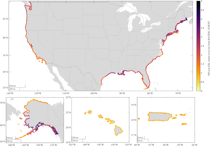
100-year return levels (m) along the coastline of the U.S., Puerto Rico and the U.S. Virgin Islands. The estimates are calculated by convolving BAYESL-TG/EXT extreme skew surge data and TPXO tidal peak distributions. All estimates are all relative to present-day mean sea level (MSL).
Fig. 3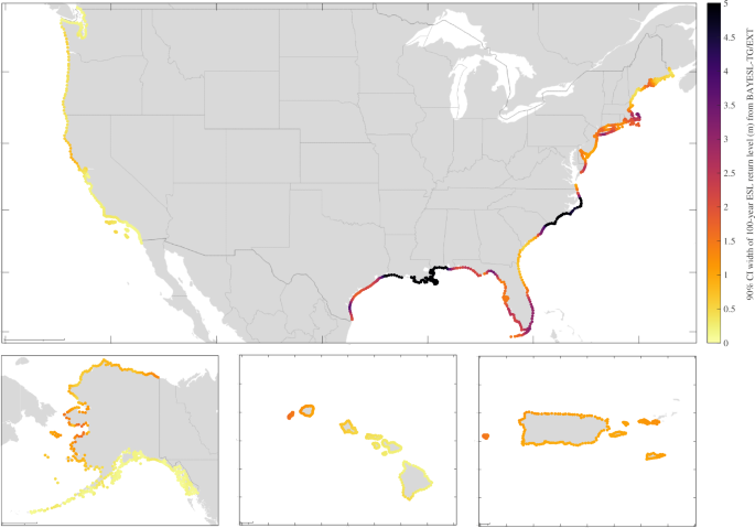
90% Credible interval (CI) width (m) associated with 100-year ESL return levels along the coastline of the U.S., Puerto Rico and the U.S. Virgin Islands. The estimates are calculated by convolving BAYESL-TG/EXT extreme skew surge data and TPXO9v5 tidal peak distributions. The latitude and longitude scales are as in Fig. 2.
Fig. 4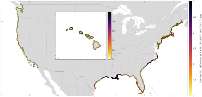
Absolute difference (m) between 100-year ESL return level estimates derived from BAYESL-TG and BAYESL-TG/EXT along the coastline of the U.S including Hawaii. The estimates are calculated by convolving BAYESL-TG and BAYESL-TG/EXT skew surge data with TPXO9v5 tidal peak distributions. The latitude and longitude scales are as in Fig. 2.