
The aim of this study was to test empirically for a general detectable fingerprint of anthropogenic drivers on the geographical distribution of human outbreaks of 32 emerging infectious diseases, based on existing geolocated outbreak and case data sources, and gridded datasets representing key socio-environmental disease drivers. To account for differing ecological characteristics across diseases and avoid testing for spurious or irrelevant associations, we generated a set of hypothesized key drivers for each individual disease through a participatory form-based exercise completed by most co-authors, whose disease-specific expertise spans a wide range of disciplines and scales of enquiry (from virology, to ecology, to global public health). Across all diseases overall, and individually per disease, we applied a standardized statistical inference framework, which involved harmonization of point and polygon data and inference of the drivers of outbreak risk using geospatial logistic regression models. We describe these methodological stages in detail in the following sections.
Collection and harmonization of geolocated human disease data
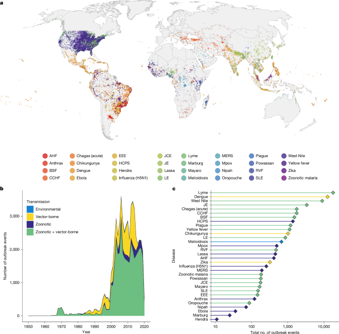
We collated and harmonized geolocated point and polygon data on human case occurrence and/or incidence of 32 environmentally linked emerging infectious diseases, from numerous published datasets in the scientific literature and from open national disease surveillance data portals (Fig. 1, Extended Data Table 1 and Supplementary Table 1). We used the following broad criteria to select diseases for inclusion: (1) human infection risk should be coupled closely and thus, in principle, attributable to local environmental or ecological conditions (that is, transmission should be zoonotic, vector-borne or environmentally mediated), and if extended human-to-human transmission chains independent of these conditions are possible, datasets must specify the locations of probable index cases. (2) Diseases should not be sufficiently well-surveyed that prevalence surveys, rather than case incidence or occurrence, could form the basis for inference. (3) Diseases should not have been subject to long-term eradication programmes that could confound inference of environmental drivers. These criteria meant that our analyses included many emerging, rare and high-concern zoonotic and vector-borne pathogens (including many mosquito-borne arboviruses, rodent- and bat-borne viruses and Plasmodium knowlesi zoonotic malaria), but not Plasmodium falciparum or Plasmodium vivax malarias or neglected tropical helminthiases.
The full list of diseases, data sources and their spatial and temporal coverage is provided in Extended Data Table 1. When compiling data for each disease, our priority was to select datasets that covered as much of the known geographic extent of transmission as possible, while remaining internally consistent (that is, collated in a standardized and comparable way to facilitate analysis). We focused on compiling existing published datasets from scientific literature and openly accessible disease surveillance portals, rather than collecting additional data (for example, by scraping scientific literature or ProMED), to ensure that our analyses are representative of data that are currently in the public domain and relatively analysis ready. Notably, sufficient or suitable data were not available for certain high-priority diseases, most notably SARS-related coronaviruses, because too few confirmed spillover events have been documented to provide a geographic picture of risk60. Datasets were obtained either by downloading from scientific paper supplementary data or open repositories, sharing between study co-authors, or through email requests to specific paper lead authors. To credit the substantial work involved in compiling the source datasets and ensure our author team included disease-specific expertise, lead authors who collated and shared datasets were invited to be study co-authors and participate in hypothesis generation (see ‘Disease-specific hypotheses for the drivers of human infection risk’) and manuscript writing and editing (see ‘Author contributions’ for a breakdown of roles).
Human case datasets are generally available in one of two formats. (1) Geolocated spillover or outbreak occurrences. Here, records represent one or more cases occurring at a named place and time, with geographical precision ranging from a specific point location or point with buffer radius (more precise), to a named administrative unit (less precise). This category of data includes most of the datasets collated for the purpose of risk mapping61,62,63,64,65,66,67,68,69,70,71,72,73,74,75,76. (2) Case counts from named areal units. Here, records contain the number of cases reported from a particular areal unit (usually first or second-level subnational administrative divisions) during a particular time window (usually a month or year). This category includes mainly datasets collected and reported through national notifiable disease surveillance systems, which are often available through online portals, reports or scientific papers. Point locations can provide greater geographic precision on environmental conditions nearby to a reported disease case, whereas administrative units require averaging conditions across often much larger polygons. Consequently, different sources provide different levels of information about both transmission intensity (binary outbreak occurrence versus number of cases) and environmental context (specific event location versus broad aggregated unit).
To ensure that the results of our models were comparable across diseases and datasets (Extended Data Table 1), we developed a harmonization framework to accommodate these diverse data sources while preserving spatial uncertainty in location of infection. A diagram of this pipeline is shown in Extended Data Fig. 1 and described as follows. The response variable, an ‘outbreak event’, was defined as at least one case in a named locality in a specified year, to ensure comparability in analyses between geolocated outbreak datasets (which contain no or partial information about the number of cases) and surveillance data (which typically provide an estimate of disease incidence). For any given disease, all outbreak locations (whether originally point or polygon) were converted to polygon objects using the ‘sf’ package v.1.0.23 in R77, by drawing a circular buffer around point locations with a radius of either 5 km, or another custom value if specified within the source dataset. This buffer size was chosen to retain a relatively high degree of spatial precision for linking point locations to environmental covariates, and assumes that infection events occurred near to where they were reported and geolocated (see ‘Limitations of data and methodology’). All polygons covering too large a spatial area were excluded as too imprecise to link to local environmental conditions; this was by default greater than 5,000 km2 (equivalent in area to a circular buffer with a radius of 40 km) but was relaxed to higher values (mostly under 10,000 km2, but maximum 20,000 km2) for certain data-sparse diseases and coarser areal case surveillance datasets (Brazilian spotted fever, chikungunya, Eastern equine encephalitis, influenza (H5N1), JCE, Marburg virus disease, Mayaro fever, Oropouche fever, plague, RVF, SLE, West Nile fever and yellow fever), as a compromise to retain as complete a geographical picture of outbreak event distributions as possible.
For each disease, this process produced a dataframe where each row with a unique identifier represents an outbreak event (that is, 1 or more cases in a given locality in a given year) with metadata where available (number of cases, case definition, diagnostic method, etc), along with an associated shapefile linking each record to a geographical polygon. For most diseases the shapefile contained a mixture of smaller circular buffers around point locations (with radius between 5 and 20 km) and larger, irregularly shaped administrative unit polygons. This variation in spatial uncertainty associated with infection events means that environmental covariates were necessarily averaged across varying geographic areas (see below), which is a feature inherent to most analyses of aggregated disease surveillance data78. We found that mean covariate values were correlated highly across a representative range of buffer sizes (Pearson’s rho > 0.8), suggesting that this issue is unlikely to substantially impact our model results (Supplementary Fig. 4).
Across all diseases, the full database contained 58,319 unique georeferenced outbreak events, for 32 diseases, in 169 countries worldwide (Fig. 1). Most records (88.7%) were from after 2000 and very few records (2.4%) were from before 1980. Most outbreak events were associated originally with spatial polygon data (73.1%), and the remaining 26.9% with point locations. The constraints of available data mean that these datasets are necessarily presence-only (that is, contain only information on positive case detections without true negatives as controls), so later modelling analysis required the selection of background points as pseudo-controls (Extended Data Figs. 1 and 2; see ‘Statistical modelling’).
Disease-specific hypotheses for the drivers of human infection risk
Many studies have proposed that certain anthropogenic changes may act as shared drivers of risk across numerous zoonotic, vector-borne and environmentally mediated diseases (for example, agriculture and urban expansion, deforestation, wildlife hunting, biodiversity loss). Yet, given their wide diversity of reservoir hosts and transmission ecologies, disease drivers may often be pathogen- or context-specific. We therefore identified sets of hypothesized drivers to test for each individual disease, to ensure our analyses accounted for expected ecological differences between systems, and to avoid identifying spurious or implausible drivers for any given system (for example, West Nile disease and wildlife hunting). Such an issue could otherwise feasibly arise owing to the small size and spatially biased nature of many disease datasets (see ‘Limitations of data and methodology’).
First, we developed a list of 18 specific socio-ecological factors that are considered principal proximal drivers of emerging disease outbreaks, including social/socioeconomic factors, human–animal contact interfaces including food systems, landscape structure, anthropogenic stressors on ecosystems and climate change. This list was developed by the lead author team who have extensive expertise in zoonotic, vector-borne and emerging diseases (R.G., S.J.R. and C.J.C.) and aimed to include as diverse and representative as possible a set of drivers, while excluding those whose influence is probably too dynamic to be detectable within spatial outbreak data (for example, extreme climate events and wildfires). The final list included ecological and landscape factors (forest and cropland cover, landscape fragmentation, biodiversity loss, invasive species), anthropogenic land use intensity and human–wildlife contact (cropland expansion, mining, protected area coverage, urban cover and expansion, wildlife hunting, wildlife trade and markets), climate change (long-term changes in temperature and precipitation), and social processes that influence exposure and/or detection (socioeconomic vulnerability, proximity to hospitals/clinics, livestock density).
Next, we identified key hypothesized drivers to test for each disease system, using a participatory exercise that was completed by study co-authors. This was conducted as a team-wide exercise, both to take advantage of the diversity of disease-specific expertise across the study authorship, and to avoid the potential for biases if hypotheses were developed by only one or a few analysts. Owing to the geographically dispersed nature of the author team, this was designed as an online form with detailed instructions. The form was structured as a fill-in matrix spreadsheet of 18 drivers and 34 disease systems (the form and instructions are provided in Supplementary Table 2). Each cell could be filled in by each author indicating their choice (four choices) of a driver having a negative, positive, none or ‘don’t know’ impact, and authors were also asked to provide a ranking (1–3) for their expected top three drivers for each disease (in either direction). Because authors have research backgrounds in different diseases, they could opt out of completing the exercise for any disease system (by leaving these blank; NA), to ensure they only selected hypotheses for diseases for which they considered they had sufficient expertise (Extended Data Fig. 5). The form was developed by two lead authors (S.J.R. and C.J.C.) and tested independently by a co-author that was not involved in the form design (C.A.L.) to ensure instructions were clear and unambiguous. This exercise was completed independently by 25 of the 31 study authors (Extended Data Fig. 5), with 6 non-participants either because they were unavailable when the exercise was conducted (3), joined the authorship after the exercise was conducted (1) or do not have infectious disease-specific expertise and instead contributed to covariate design (2). None of the authors had seen the combined dataset or preliminary results before completing the exercise, except the lead analysts (R.G., C.J.C.) who had seen preliminary results for three diseases during pipeline development (Ebola, Lassa, CCHF) but not the results of fully adjusted models with geospatial and detection effects.
The authorship includes members with significant expertise and disease-specific publications for most of the infections included in this study, including anthrax, rodent-borne arena- and hantaviruses, Chagas disease, urban Aedes-borne arboviruses, zoonotic mosquito-borne arboviruses, CCHF and other tick-borne infections, avian influenza, bat-borne henipaviruses and filoviruses, Lyme disease, melioidosis, MERS, mpox and related orthopoxviruses, and plague. The group has a diverse set of disciplinary backgrounds, including disease ecology and evolution, epidemiology, microbiology and virology, genomics, veterinary medicine, social-ecological systems and public health. Nonetheless, our team still consists largely of academic researchers based in Global North institutions, and as such our hypotheses are unlikely to fully reflect locally situated understandings of most of these diseases. Although this online exercise was a concise approach to participatory hypothesis development across an international author team, authors still reported spending several hours (more than 2 h) to fully complete the matrix, so we cannot recommend this current design as the basis for a large-scale survey.
We then postprocessed the completed exercise data to generate lists of hypothesized drivers to test for each disease, based on three different levels of stringency for author agreement, as a sensitivity test to ensure our approach did not introduce systematic bias in the findings. We first adopted a moderate stringency criterion, including drivers for which more authors stated an effect (either positive or negative) than stated no effect (‘majority rule’); this retained 80% of disease–driver combinations to test. We also adopted a high-stringency criterion, including only drivers that were included in the top three ranked drivers by at least one author (‘top-ranked’; retaining 50% of disease–driver combinations), and a lowest stringency criterion, including all drivers for which at least one author had stated an effect (‘any author’; retaining 97% of disease–driver combinations). The ‘any author’ criterion tests nearly all potential relationships, excluding only extremely implausible drivers, so under this criterion the results are driven primarily by the patterns within the data, with minimal influence of the hypothesis exercise. The study results were quantitatively and qualitatively very similar under these three criteria, indicating that our findings were not biased systematically by the hypothesis exercise. We present results using the ‘majority rule’ criterion in the main figures, as this criterion reflects the balance of author agreement, and present results for the other criteria as Supplementary Information (Supplementary Figs. 2 and 3).
Collation of geospatial data on socio-environmental drivers of disease
In parallel, we collated global geospatial (raster) layers describing socio-environmental and climatic features as proxies for the key geographic drivers of risk listed above, based on remote sensing, climate reanalysis, social indicators and census-based data sources. A full table of socio-environmental covariates, their sources and processing is provided in Extended Data Table 2 and Supplementary Table 3. The small size of many disease datasets unfortunately meant there was insufficient data to analyse the relationship between cases and covariates in both space and time, which therefore limited our study to spatial rather than spatiotemporal driver analysis (see ‘Limitations of data and methodology’). Therefore, for variables describing gross characteristics of the environment (for example, land cover type proportion variables) we selected a single raster year or time period close to the central tendency of reported disease data (between 2005 and 2015), while aiming for gridded products that provide the best spatial and thematic resolution possible under that constraint. For variables describing anthropogenic change, we generated rasters that described the grid-cell-level change in a particular variable across most of the disease data period (for example, tree cover loss between 2000 and 2020, change in mean annual temperature between 1950–1970 and 2000–2020). Raster covariates were used at their original spatial resolution with a few exceptions (for example, social vulnerability was aggregated; Extended Data Table 2); as this was not a mapping study, no rescaling was required. In all cases a key criterion was, wherever possible, to use global raster products that were comparable across regions and diseases. For most drivers there was a natural match to proxy covariate metrics (for example, percentage land cover variables, average climatology change from a historical reference, livestock density, cumulative tree cover loss, cropland or urban expansion); we selected ERA5-Land for climate owing to its rich historical coverage and high accuracy, and Copernicus land cover for land cover variables owing to its combination of high spatial and thematic resolution. For other drivers, we selected the only available globally comparable spatial product (Biodiversity Intactness Index; Global Relative Deprivation Index). Certain drivers involved choosing a specific product over other options: we selected the modelled hunting pressure index for tropical forests79 owing to its clearly reported modelling approach and its geographic extent, which was larger than that of other hunting pressure maps; and we selected EVI dissimilarity from ref. 80 as a landscape heterogeneity metric, because the original study showed this metric was sensitive to anthropogenic fragmentation and correlated strongly to biodiversity metrics (so a suitable proxy for the ecological dynamics of fragmented landscapes). Notably, we were unable to identify suitable proxy covariates for several widely hypothesized drivers that have not been quantified in space and time, highlighting an important lack of systematic spatial data collection around key putative drivers of disease emergence; these include invasive species density, wildlife trade and/or live markets, and wildlife hunting outside tropical forests.
A brief description of the full list of the socio-environmental raster datasets is as follows: temperature change (change in grid-cell-level mean annual air temperature between reference period of 1950–1970 and focal period of 2000–2020, derived from ERA5-Land reanalysis81); precipitation change (change in grid-cell-level mean annual precipitation between 1950–1970 and 2000–2020, from ERA5-Land); forest cover (grid-cell-level fractional tree cover from Copernicus land cover 2015); forest loss (grid-cell-level tree cover loss 2000–2020 from Global Forest Change); biodiversity intactness (local Biodiversity Intactness Index, that is, the predicted average local abundance of all species relative to their abundance in minimally disturbed habitat, for 2005 based on human disturbance layers82); cropland cover (grid-cell-level fractional crop cover from Copernicus land cover 2015); cropland expansion (grid-cell-level cropland growth 2000–201983); landscape heterogeneity (grid-cell-level second-order EVI dissimilarity index 2005, a metric of landscape fragmentation sensitive to anthropogenic landscapes80); hunting pressure index (a modelled defaunation index measuring average hunting-related species declines in tropical forest biomes79); protected area cover (whether grid cell is under area-based conservation, based on the World Database of Protected Areas 2022); mining cover (whether grid cell is under mining land use, based on ref. 84); social vulnerability (the Global Gridded Relative Deprivation Index, a composite indicator based on inputs including infrastructure, human development index, nighttime lights and infant mortality rate, for a nominal present-day period85); travel time to healthcare (road-based travel time to nearest hospital or clinic for nominal year 201555); urban cover (grid-cell-level fractional urban cover from Copernicus land cover 2015); urban expansion (grid-cell-level expansion of built-up areas 2000–2019 derived from ESA-CCI land cover); and livestock density (grid-cell-level density of livestock types from Gridded Livestock of the World v.3).
Statistical modelling
To infer the drivers of the geographic distribution of human cases while accounting for spatial and detection biases, we applied a standardized geospatial modelling approach for each disease.
For each model, we first defined the geographical boundaries of the modelling area (‘study region’). For datasets compiled from the scientific literature, this was defined as a smoothed convex hull polygon around the full extent of geographical case occurrences, with a buffer of 180 km (Extended Data Figs. 1 and 2). For national-level case surveillance data the study area was constrained to the borders of the relevant country or subnational region. We then generated a final case-control dataset for modelling. We excluded records from before 1985 for most diseases, to better align the disease data with the timescale of available covariates; exceptions were certain data-sparse diseases where data from after 1980 were included, to retain as much information as possible (anthrax, Ebola virus disease, Marburg virus disease, Mayaro fever and Oropouche fever).
Because the case data were presence-only, meaning there were no true negative controls, we then generated background (pseudo-control) points throughout the study region. We selected between two and eight times as many background points as presence points, with the aim of ensuring sufficient coverage of the background area while balancing against computational costs. The higher numbers were selected for diseases that had a low number of outbreak points across a large study area (for example, Oropouche, Ebola) to ensure coverage of the full study area, whereas the lower numbers were selected for diseases with a large number of outbreak points across the study area (for example, Lyme, West Nile). (Various guidelines have been proposed for background points selection to maximize predictive performance in species distribution models86, but our study objective is inference of driver effects rather than optimizing for prediction; as such, our priority is statistical power and coverage of the study region for each disease). All else being equal, the null expectation is that the distribution of human disease cases would follow the distribution of population; as such, entirely spatially random selection of background points would over-represent sparsely populated rural areas and under-represent highly populated urban areas. Therefore, we weighted background points distribution by human population, that is, randomly generated point locations with the probability of a location being selected proportional to log+1-transformed population. This was based on a global raster of 2010 human population per pixel (WorldPop’s top-down unconstrained mosaics87), at 1-km resolution for most diseases, but 10-km resolution for certain diseases spanning a multi-continent geographic range to limit computation time (for example, dengue, chikungunya). This approach produced a pseudo case-control design, that is, comparing the socio-environmental conditions experienced by human populations at the locations where outbreaks have occurred (cases) with a representative background sample of the conditions experienced by populations across the study region (‘controls’). Circular buffers were created around each background point with an area equal to the median area of the outbreak location polygons, to ensure covariates were averaged across a comparable geographical area for both presence and background points (Extended Data Fig. 1).
For each model, this process produced a final dataframe of presences and pseudo-absences with associated polygons (again using ‘sf’), from which we extracted the mean value for each raster covariate using the package ‘exactextractr’ v.0.10.1. We excluded from the analyses any variables that were missing data for greater than 10% of observations or contained zeroes for greater than 95% of observations. We examined collinearity among covariates using visual inspection, correlation matrix plots and variance inflation factors, and identified and excluded highly collinear covariates from multivariable models; this step was conducted manually rather than programmatically, to prioritize the inclusion of covariates with a stronger hypothesized relationship to each disease in question (based on the ‘majority rule’ hypothesis list). The final sets of covariates included in each disease-specific multivariable model are visualized in Extended Data Fig. 6.
To infer relationships between covariates and disease outbreak probability P at location i (log odds of occurrence), we fitted geospatial logistic regression models in a Bayesian inference framework (integrated nested Laplace approximation, implemented in the package ‘INLA’ v.23.3.26 (refs. 88,89)), with the following general formula:
$$\begin{array}{c}{y}_{i} \sim {\rm{B}}{\rm{e}}{\rm{r}}{\rm{n}}({p}_{i})\\ {\rm{l}}{\rm{o}}{\rm{g}}{\rm{i}}{\rm{t}}({p}_{i})=\alpha +{\rho }_{i}+\sum _{j}{{\boldsymbol{\beta }}}_{j}{X}_{j,i}\end{array}$$
Here, \(\alpha \) is the intercept, \({\rho }_{i}\) is a continuous spatially structured random effect and β is a vector of linear fixed effects parameter estimates for the matrix of \(j\) covariates \({X}_{j}\). The geospatial effect was specified as a Gauss–Markov random field fitted using a stochastic partial differential equations approach, with penalized complexity priors on the range and sigma parameters and an intermediate mesh density chosen to balance reasonably between spatial precision and computation time. We set Gaussian priors for intercept and linear fixed effects (mean = 0, precision = 1). Different diseases varied widely in both geographic range size and patchiness of data, so to avoid issues with overfitting or underfitting of the spatial field, for each disease we manually adjusted the hyperpriors for the stochastic partial differential equation model’s Matern covariance function (range and variance hyperparameters) to ensure that the spatial field was fitted smoothly to the spatial structure of the outbreak event data (that is, there were no visible issues with inference of the geospatial effect; Extended Data Fig. 2). After model fitting, we then extracted the Watanabe–Akaike information criterion as a comparison metric of model fit.
Global multi-disease models
We first fitted general models to infer drivers of risk for all disease outbreaks—not differentiating between diseases—using the full dataset of 49,239 outbreak events (after excluding early and spatially imprecise records) and 50,000 population-weighted background points across the global study area. The extreme imbalance in sample sizes between different diseases (Fig. 1) could lead to estimates being biased by well-represented diseases. To avoid this issue, we estimated fixed effects posterior distributions for each driver from an ensemble of 100 submodels fitted to balanced subsamples of the data. Each submodel was fitted to a dataset including 100 randomly subsampled outbreak points per disease (all outbreak points for any diseases with fewer than 100 points in total), and twice as many randomly subsampled background points. We drew 1,000 posterior samples per fixed effect from each submodel, then calculated credible intervals (median, 67% and 95% intervals) using pooled posterior samples from all 100 submodels. This approach ensured a balanced representation of data across all diseases when inferring overall driver effects. We applied this ensemble approach for each of the models described in the following paragraph, but for simplicity we refer to the pooled results from each ensemble as a ‘model’.
To examine the potential confounding effects of local detection processes and broad-scale patterns of reporting effort on inferred drivers, we fitted three global models: (1) including only socio-environmental covariates, that is, with no outbreak detection-specific covariates (urban cover and healthcare travel time) and no geospatial effect; (2) adding a geospatial effect but no local outbreak detection-specific covariates; and (3) a full model with outbreak detection covariates and a geospatial effect (Fig. 2). For comparison and sensitivity checking by transmission pathway, we also fitted the full geospatial and detection covariate model for subsets of pathogens defined as either zoonotic (principally transmitted to humans from an animal reservoir; n = 26) or vector-borne (transmitted to humans by arthropod vectors irrespective of host, that is, also including anthroponotic arboviruses such as dengue fever; n = 20), whose risk is expected to be coupled tightly to local ecosystem characteristics (Extended Data Fig. 3a). Given the significant regional variability in the intensity and correlation structure of emerging disease drivers (Extended Data Fig. 4), we also fitted five models to data from different geographic regions (North America, Latin America and the Caribbean, Sub-Saharan Africa, South Asia and East Asia and the Pacific), to examine the consistency of inferred drivers across these varied socio-ecological contexts (Extended Data Fig. 3b).
Individual disease-specific models
We fitted individual models for all diseases except Hendra virus disease, for which the number of human outbreak points was too low for reliable model fitting (Extended Data Table 1). The process of inferring drivers for each individual disease (n = 31) was as follows. First, we fitted separate geospatial models which included each covariate individually (‘univariable’) plus a geospatial random effect to account for the broad geographical pattern in outbreak occurrence, but not possible finer-scale confounding by other variables (particularly detection proxies). We then fitted three separate hypothesis-driven multivariable geospatial models including drivers identified using the three filtering criteria from the co-author exercise (majority rule, top-ranked and any author) (Extended Data Fig. 5). Because of the strong a priori expectation of detection bias driven by health systems proximity and accessibility, all multivariable models included both travel time to healthcare and urban cover; except in instances where these were highly collinear with each other; in these cases, the driver identified as most important in the hypothesis-generation exercise was selected. For all models where forest loss, cropland expansion or urban expansion were hypothesized as drivers, we also included either forest cover, cropland cover or urban cover, respectively, to account for the inherently spatially correlated process of land use change. For most diseases, urban expansion and urban cover were highly collinear at the scale of this analysis (Pearson’s P > 0.8) so urban expansion was almost always excluded from multivariable models. For diseases with strongly hypothesized associations to specific livestock, the livestock covariate was based on gridded data for only the most relevant livestock type(s) (for example, poultry for influenza, ruminants for RVF; Supplementary Table 1 and Methods); the exception was MERS, as gridded camel density data are not openly available. Across all diseases, the hypothesis-driven multivariable models always reduced Watanabe–Akaike information criterion relative to a model including only a geospatial effect (including covariates improved model fit). For the two diseases with sufficient data coverage in more than one global region (dengue in the Americas, Africa and Asia; yellow fever in Latin America and Africa) we also fitted region-specific multivariable models to examine the consistency of inferred drivers across different socio-ecological settings (Extended Data Fig. 8).
Examining aggregate and shared driver effects across disease groups
For many infectious diseases, synergistic interactions between drivers may be necessary to align the conditions for spillover and emergence risks (for example, high livestock densities in fragmented forest landscapes for bat-borne henipaviruses6). Improving geospatial prediction for emergence risks requires accounting for how compound drivers align to create local foci of pathogen transmission. To examine this question we estimated the mean effect size for each driver and visualized patterns of co-occurrence between drivers, across all 31 individual modelled diseases, and for subsets of either directly transmitted (n = 10) or vector-borne (n = 17) zoonoses. For each driver, we generated a posterior distribution of the mean effect size across all diseases for which that covariate was tested. To achieve this, we calculated the mean fixed effect size using one randomly drawn posterior sample from each tested disease, and repeated this 5,000 times for each driver to build up a posterior distribution, from which we calculated median, 67% and 95% credible intervals (Fig. 4a–c). The resulting mean effect distribution therefore explicitly incorporates the variation in fixed effects uncertainty between different diseases (owing to differences in sample size and variability), with wider posterior intervals reflecting more heterogeneity in effects directionality and/or greater statistical uncertainty. We only conducted this analysis for drivers that were tested for five or more diseases, to ensure our mean estimates were not overly biased by a very small sample of diseases.
To visualize the pattern of shared drivers, we generated unipartite networks with drivers represented as nodes, and with edges between driver pairs weighted by the number of diseases for which each pair of drivers co-occurred (when both drivers had 95% credible intervals not overlapping zero; Fig. 4d–f). In parallel, to examine observed autocorrelation among putative drivers at global and regional scales, we generated a matrix of pairwise Pearson correlation coefficients between each pair of scaled covariates across 50,000 background points globally, or subsets of background points within five regions containing most of our data (North America, Latin America and the Caribbean, sub-Saharan Africa, East Asia and Pacific, and South Asia). These were used to visualize unipartite networks of pairwise driver correlations, with edges weighted by Pearson coefficient magnitude (Extended Data Fig. 4).
Limitations of data and methodology
Because the goal of the study was to apply a general, standardized analysis framework across a variety of diseases with very different quantities and types of data, we encountered several important but irreconcilable methodological constraints that are significant to interpretation of our results, as well as to inference of spatial drivers of disease emergence more broadly. First, the datasets for many diseases (especially rare and high-consequence pathogens) are very small and spatially biased towards surveillance hotspots. We adjusted for these biases using geospatial random effects and proxies for detection processes, but these are imperfect descriptors for complex processes, and some residual confounding might remain unaccounted for (for example, health systems access is influenced locally by many factors other than proximity, and clinical index of suspicion and accessibility of diagnostics is often highly geographically variable for many rarer, non-specific febrile illnesses). Relatedly, it was often not possible to combine several data sources for the same disease without creating a geographical imbalance in the distribution of points, so our analyses were restricted mostly to datasets that were usually broad in scale but lacked granular information about transmission intensity (for example, most georeferenced outbreak datasets) or sometimes locally comprehensive at the expense of geographical breadth (for example, HCPS, which was restricted to Brazil and Argentina owing to available surveillance data, despite hantavirus infections occurring worldwide90). Notable exceptions where we were able to combine point and polygon data from more than one source without substantial issues included Lassa fever, CCHF, HCPS, Chagas disease (acute) and yellow fever (Extended Data Table 1 and Supplementary Table 1).
Some of the most relevant variables thought to shape risk for many high-consequence epidemic zoonoses either have not (hunting pressure outside the tropics) or cannot (wildlife trade) be translated readily into global geospatial covariates that accurately reflect their relationship to infection risk. For example, the impacts of wildlife trade and markets on disease risks can be spatially diffuse and transboundary, involving several actors at several points along commodity chains from capture to sale91; consequently, quantifying how these activities shape the spatiotemporal dynamics of zoonotic spillover may require substantially different analytic approaches than what is possible with this study’s geolocated outbreak event data. (However, we also refer to other work that has highlighted instances where wildlife trade has been overstated as a driver of spillover risk15.) Similarly, coarse modelled spatial proxies for hunting pressure such as the tropical defaunation index we used in this study79 probably more closely reflect commercial rather than subsistence hunting activities, even though the latter may often be more important in driving zoonotic spillover (for example, rodent hunting and exposure to Lassa fever and mpox); our study’s sparse and ambiguous results for tropical hunting pressure (Extended Data Fig. 6 and Supplementary Fig. 1) should be interpreted with this limitation in mind.
Developing a common analysis framework also led to the loss of information from some datasets, through reducing case surveillance data (with number of cases) to a binary annual outbreak indicator (losing potentially valuable information on transmission intensity). Although necessary for a standardized framework, this could feasibly erode the reliability and accuracy of inference. We therefore conducted a model comparison test, examining how reducing the data’s information content affects inferred drivers for a set of relatively well-reported diseases (four arboviruses in the continental USA using CDC ArboNET data). For each disease we compared coefficient estimates between full geospatial models of county-level case incidence, and our outbreak event risk modelling framework. County-level total case incidence across the surveillance period (2000–2020) was modelled using a negative binomial (West Nile fever) or zero-inflated negative binomial likelihood (La Crosse encephalitis, Powassan encephalitis and JCE), including an offset of log population, and a fitted geospatial random effect to account for unexplained geographical variation, again implemented using INLA. We found that most significant socio-environmental effects from a full case incidence model (reflecting transmission intensity) remained detectable even in a dataset reduced to binary outbreak occurrences with background locations (Extended Data Fig. 7). This test improved our confidence that our modelling approach is sufficient to capture key spatial drivers of risk, despite this information loss.
Nonetheless, given data sparsity for many infections, it was not possible in this standardized framework to account for temporal dimensions of causality (for example, time-specific climate or land change effects), such as by aligning covariate and case data in time, and/or adjusting for temporal patterns of detection through spatiotemporal random effects. This kind of analysis is feasible and fruitful when modelling case surveillance time series for better-surveyed infections (including some in our study such as Lyme disease or West Nile fever), but it was not possible to apply this consistently across diseases, given the extreme sparsity of outbreak data for infections such as Ebola, Marburg, Hendra and Nipah virus disease. Data sparsity also prohibited explicitly testing for nonlinear effects of drivers, although we sought to mitigate this issue by selecting covariates for individual processes whose monotonic effects combine to produce apparent nonlinear effects (for example, habitat loss and fragmentation acting together to produce peaks in spillover risk at intermediate levels of land conversion37). The lack of fine-scale spatiotemporal data also meant we could not disentangle elevated outbreak detection rates in urban areas, from the potential true contribution of urban social and environmental processes to risk for certain diseases; for example, human population density and urban mosquito habitats may play a significant role for Aedes mosquito-borne viruses that transmit between humans (dengue, chikungunya and Zika). Nonetheless, we do not expect consistent positive relationships between human density and spillover risk across all diseases in our data (many of which have rural sylvatic ecologies). Rather than solely a limitation of this study, these are more general problems for attribution of outbreak drivers for rarely documented but high-consequence infections, that currently hinders our capacity to, for example, robustly link recent deforestation to viral zoonosis outbreaks. Improving both fundamental eco-epidemiological research, and strengthening healthcare access, diagnostics and surveillance in underserved areas, will be needed to fill these gaps.
Reporting summary
Further information on research design is available in the Nature Portfolio Reporting Summary linked to this article.