
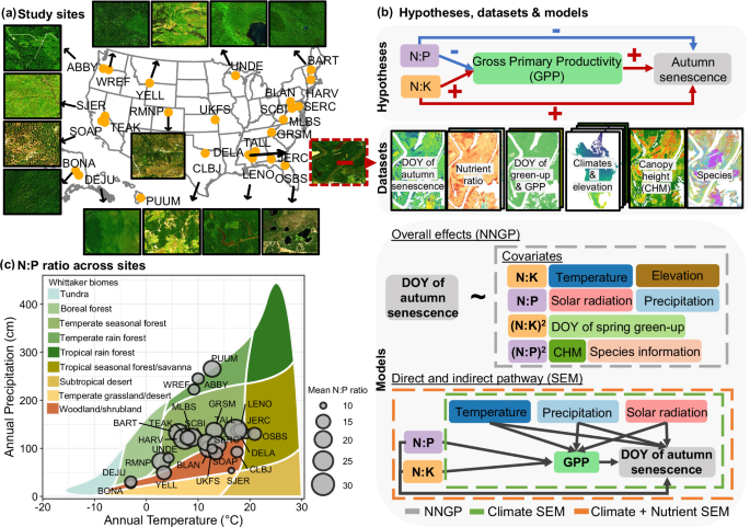
Study sites
We quantified the effects of canopy nutrient ratios (i.e., N:P and N:K) on autumn senescence using all NEON sites with available canopy nutrient maps and more than 50% woody vegetation cover (n = 25; Fig. 1a). Woody cover was estimated from the National Land Cover Dataset (NLCD), including deciduous forest, evergreen forest, mixed forest, and shrub classes, and it was cross-checked with the RGB composite of the hyperspectral imagery. Each site covers an area of approximately 10 × 10 km and the 25 sites together span a broad range of climatic and biogeochemical conditions (Fig. 1a). Detailed descriptions of site characteristics and dominant forest types are provided in Table S1.
Data collection, processing, and aggregation of satellite-derived land surface phenology data
The timing of autumn senescence was obtained from the PlanetScope Land Surface Phenology (PLSP) datasets31. It was defined as the Day of Year (DOY) when greenness declined to 15% of the seasonal amplitude. The PLSP dataset31 was derived from 3 m PlanetScope imagery across the NEON network using the following steps27,43. First, daily surface reflectance was composited to compute two-band Enhanced Vegetation Index (EVI2)44, a proxy of vegetation greenness that is less prone to saturation over dense canopy cover, soil background influences, and residual cloud/snow contaminations. Second, the EVI2 time series fluctuations related to clouds, atmospheric aerosols, and snow were removed based on both Quality-Assurance layers (QA) and outlier detection criteria (i.e., negative EVI2 values) at each pixel. Third, the background EVI2 value outside the growing season was determined using the 10th percentile of snow-free EVI2 values at each pixel. It was used to fill the time series EVI2 values at any dates with EVI2 values lower than the background EVI2 or no observations during the dormant periods. Fourth, the penalized cubic smoothing splines were employed to create gap-free EVI2 time series. Phenological cycles were then identified from these curves to retrieve land surface phenology (LSP) metrics, which show strong agreement (R ≥ 0.87) with near-surface PhenoCam observations45. In addition to the date of autumn senescence, we extracted the day of year corresponding to 15% of the seasonal amplitude as spring green-up. Finally, we integrated daily EVI2 from green-up to senescence to obtain the EVI2 integral46, which we used as a proxy for GPP.
Canopy nutrient data
We obtained hyperspectral data from the NEON Airborne Observation Platform (AOP) as orthorectified surface directional reflectance products (product ID DP1.30006.001). The AOP imaging spectrometer acquires 426 bands spanning 380 and 2500 nm at 5 nm spectral resolution and 1 m spatial resolution. Although AOP provides multi-year hyperspectral coverage for some NEON sites, many flight lines contain cloud and shadow contamination. AOP flight crews evaluated the percentage of cloud cover (CC) at three levels: green (CC < 10%), yellow (10% 50%). We visually inspected all green-flagged flight lines and selected a single best-quality acquisition for each site based on minimal cloud and shadow contamination. For some large sites, the selected acquisition consisted of multiple flight dates within the same year because a single day of AOP flights was insufficient to cover the full site extent. Acquisition years and days are reported in Table S125.
Although the use of a single best-quality acquisition per site reflects a practical constraint of NEON AOP availability, these flights are scheduled to coincide with peak greenness of the growing season at each site47, and canopy nutrient ratios are expected to be more temporally stable than absolute nutrient concentrations during the growing season25. These ratios are therefore directly relevant to overall canopy physiological function and resource allocation processes that precede autumn senescence. At the same time, timing-related uncertainty in single-date nutrient maps would most likely act as measurement error in the predictor variables. Because phenology metrics were matched to the year of the selected nutrient map, we expect this source of uncertainty to be reduced. Nonetheless, nutrient concentrations can exhibit seasonal dynamics, and future work incorporating multi-temporal nutrient mapping would strengthen this aspect of the analysis.
We followed the published preprocessing and trait-mapping workflow of Wang et al. (2020)26. Surface reflectance was corrected for terrain and view–illumination effects using HyTools (v1.4)48, including topographic and bidirectional reflectance distribution function (BRDF) corrections. We removed noisy atmospheric absorption bands and retained spectral regions 418.59–1335.04 nm, 1460.23–1770.72 nm, and 1986.06–2396.71 nm, yielding an average of 354 bands across sites. We then generated wall-to-wall canopy nutrient maps by applying published partial least squares regression (PLSR) coefficients to the corrected reflectance data. The underlying PLSR models were developed and validated by Wang et al.26 using field-collected, sunlit, top-of-canopy foliar samples paired with corresponding AOP pixels across NEON sites. The calibration dataset included approximately 300 samples per trait, with canopy chemistry measured from foliar material collected during the same campaigns used to support NEON trait mapping. Wang et al.26 selected the number of latent components using repeated cross-validation with 200 permutations and used the same procedure to quantify prediction uncertainty and reduce overfitting. Full details of sample distribution, filtering, calibration, and validation are reported in Wang et al.26. Model coefficients are publicly available through the Ecological Spectral Model Library (EcoSML version 1.0; https://ecosml.org/package/github/EnSpec/NEON-Trait-Models). For canopy N, P, K, the R2 values were 0.92, 0.70, and 0.72, respectively; normalized RMSE (RMSE/data range) was 6.75%, 12.8%, and 13.24%, respectively. Because we apply these pre-trained coefficients to AOP imagery from the same NEON domain, the reported accuracies should be interpreted as in-sample predictive performance. We used both linear and quadratic terms for the canopy nutrient ratio predictors because of their potential non-linear effects on ecosystem functions11,33. The year of all other covariates (see following section) was matched to the year of each site’s canopy nutrient maps. Therefore, all analyses in this study focused on within-site spatial variation in canopy nutrients and autumn senescence within the selected site-year, rather than interannual variations. Both nutrient ratios were included in the same model. Marginal effect curves were plotted separately for visualization by varying one nutrient ratio while holding the other predictors constant.
Climate, canopy structure, and other ancillary data
We extracted mean temperature, cumulative precipitation, and cumulative shortwave radiation between the mean timing of spring onset and autumn senescence from the Daily Surface Weather Data at 1 km resolution (Daymet)49. These variables were included to control for broad seasonal climate variation within each site-year, rather than to resolve canopy-scale microclimate. We obtained elevation data at 1-meter spatial resolution from the NEON AOP products50 and vegetation structure to account for local topographic effects and microclimate variability that are not resolved by the coarser-resolution climate data. Vegetation structure complexity was characterized with canopy height model (CHM) derived from AOP’s LiDAR point cloud product51. Point clouds were ground classified to build a digital terrain model using a triangulated irregular network (TIN) algorithm; a digital surface model was then generated from first returns, and the CHM was computed as surface minus terrain. In addition, the NNGP spatial effect (see next sections) accounts for residual spatial structure that may arise from unresolved microclimate, edaphic heterogeneity, or other spatially autocorrelated drivers. Because phenology is largely influenced by species, we obtained site-level canopy tree species maps from Weinstein et al.52 where available. We used the dominant species for each grid cell as the covariate for the model. For sites lacking these species maps, we used the National Land Cover Database (NLCD)53 to distinguish broad canopy types (e.g., deciduous vs conifers). The dominant species and canopy types for each site is listed in Table S1.
Data processing and aggregation
We defined a common analysis extent for each site by intersecting all input datasets. Within this extent, we retained only high-quality pixels from the PLSP dataset (QA = 1 or 2). The QA layer is provided by the dataset and is evaluated using the correlation between observed and fitted EVI2 and the length of data gaps. To balance computational efficiency and ensure consistency among multi-source inputs, we set the analysis scale to 30 m and aggregated all layers to this resolution using the median values within each 30 × 30 m grid cell. For the 19 sites with species maps (Table S1), we excluded non-woody pixels so that modeled grid cells represented woody-dominated vegetation and minimized the influence of herbaceous phenology and chemistry on nutrient–phenology relationships. For the remaining six sites without species maps (Table S1), we retained all pixels rather than masking with the NLCD alone, because the 30 m NLCD product can miss sub-pixel woody cover and could exclude pixels that still contain substantial woody vegetation. Although this choice may permit some mixing of woody and herbaceous signals at those sites, we found no systematic differences in the magnitude or direction of nutrient–phenology relationships between more forested sites and tree–grass mosaic sites. These results suggest that the main ecosystem-scale patterns are robust, while masking based on species maps provides a cleaner delineation of woody vegetation where available. Prior to model fitting, we standardized all response variables and covariates to enable direct comparisons across sites. In total, we compiled a total of 4605–61,736 grids across the 25 NEON sites, which served as the spatial units for model training and validation.
NNGP and SEM modelingNearest neighbor Gaussian process (NNGP) model
Our previous work found that NNGP effectively captured within-site spatial variations across major U.S. biomes, achieving R2 > 0.5 at 84% of sites for spring and 80% for fall phenology29. Therefore, we fit an NNGP model within the Bayesian hierarchical framework at each NEON site54. Specifically, the NNGP model follows the structure of spatial regression model including fixed effects from covariates, a spatial random effect that accounts for unmeasured, spatial dependence that is common in remotely sensed dataset, and a noise residual term as denoted as the following equation55:
$$y({S}_{i,n})={x\left({S}_{i,n}\right)}^{{{\rm{\top }}}}\beta+\omega \left({S}_{i,n}\right)+\varepsilon ({S}_{i,n})$$
(1)
Where \(y({S}_{i,n})\) is the observed response at location \({S}_{i}\) within site \(n\), \({x\left({S}_{i,n}\right)}^{\top }\) is the environmental covariates at location \({S}_{i}\), \(\beta\) represents the regression coefficients (i.e., fixed effects), \(\omega \left({S}_{i,n}\right)\) is the spatial random effect at location \({S}_{i}\) for site \(n\), and \(\varepsilon ({S}_{i,n})\) is the location-specific random noise following a normal distribution \(N(0,\,{\tau }^{2})\) where\(\,{\tau }^{2}\) is the nugget variance.
NNGP can be expressed as a three-level Bayesian hierarchical model that partitions variations into data, process, and parameter levels55. At the data level, the observed responses can be modeled as:
$${Y|W},\,\beta,{\tau }^{2}\, \sim N(X\beta+W,\,{\tau }^{2}I)$$
(2)
Where \(Y\) is the observed response, \(X\) is the design matrix, \(W\) is the spatial random effects, and \(I\) is the identity matrix for residual noises. Note that we drop the subscript from Eq. 1 to avoid clutter.
At the process level, we modeled the spatial random effects as a Gaussian process (GP) with mean zero and spatial covariance structure in the following\(:\)
$${W|}{\theta }_{n}\, \sim N(0,\,C({\theta }_{n}))$$
(3)
Where \(C({\theta }_{n})\) is the spatial covariance matrix parameterized by \(\theta\) within site \(n\). The full GP is then replaced with an nearest neighbor GP that is a sparse approximation of the full covariance structure54,55, which improves the computational efficiency:
$$W \sim {NNGP}(0,C({\theta }_{n}))$$
(4)
$$C\left({\theta }_{n}\right)=C\left({S}_{i,n},{S}_{j,n};{\theta }_{n}\right)$$
(5)
Where \({S}_{i,n},{S}_{j,n}\) indicate two locations \({S}_{i}\) and \({S}_{j}\) within the same site \(n\). We used the exponential covariance function to define \(C({\theta }_{n})\):
$$C\left({S}_{i,n},{S}_{j,n};{\theta }_{n}\right)={\sigma }_{n}^{2}\exp (-d\left({S}_{i,n},{S}_{j,n}\right)/{\varphi }_{n})$$
(6)
where \({\sigma }_{n}^{2}\) is spatial variance representing overall variance within site \(n\), \({\varphi }_{n}\) is range parameter controlling how fast correlation decays, and \(d({S}_{i,n},{S}_{j,n})\) is distance between location \({S}_{i,n}\) and \({S}_{j,n}\).
At the parameter level, we assigned prior distributions to all model parameters, including \(\beta\), \({\tau }_{n}^{2}\), \({\sigma }_{n}^{2}\), \({\varphi }_{n}\), and \({\theta }_{n}\). The posterior distributions are obtained using Markov chain Monte Carlo (MCMC) sampling55.
Model fitting and validation
We used R package spNNGP55 to fit the NNGP model. The response was the DOY of autumn senescence. The environmental covariates included the linear and quadratic terms of the summer canopy N:P ratio and N:K ratio, climate variables during the growing season (i.e., mean temperature, cumulative precipitation, cumulative shortwave radiation), the timing of spring green-up, elevation, and CHM. We also included the dominant species as a categorical variable. While dominant species or broad canopy type was included as a categorical variable to account for major taxonomic differences in phenology and nutrient strategies, we recognize that finer-scale species composition and intra-specific variability within 30 m grid cells could introduce additional heterogeneity not fully captured by this broad categorization. This inherent complexity of natural forest stands may contribute to some of the unexplained variance or site-specific patterns observed.
Regression coefficients were assigned the default flat prior implemented in spNNGP package, \(p\left(\beta \right)\propto 1\), which can be viewed as the case of a Normal prior with variance tending to infinity. For spatial covariance parameters, including the spatial decay parameter (\({\varphi }_{n}\)), spatial variance (\({\sigma }_{n}^{2}\)), and nugget variance (\({\tau }_{n}^{2}\)), we specified common weakly informative priors across sites. We first plotted empirical semi-variograms as exploratory diagnostics and found that\(\,{\tau }_{i}^{2}\) was generally near zero, \({\sigma }_{n}^{2}\) ranged from approximately 0.5 to 1, and the spatial decay \({\varphi }_{n}\) corresponded to distances from a few hundred to roughly thousands of meters. We assigned \({\varphi }_{n}\) a uniform prior, \({\varphi }_{n}\sim U(3/{\mathrm{2000,3}}/1)\), which spans very fine-scale to kilometer-scale residual spatial structure under the exponential covariance parameterization. Spatial variance and nugget variance were assigned inverse-gamma priors, \({\sigma }_{n}^{2}\sim {IG}({\mathrm{2,0.5}})\) and \({\tau }_{n}^{2}\sim {IG}({\mathrm{2,0.5}})\), respectively. The semi-variograms were used only to verify that the common prior range was computationally reasonable; they were not used to construct site-specific priors. The inverse-gamma priors on \({\sigma }_{n}^{2}\) and \({\tau }_{n}^{2}\) are conditionally conjugate for the Gaussian variance components; the spatial decay parameter \({\varphi }_{n}\) is not conjugate and is updated within the MCMC algorithm implemented in the package.
We randomly selected 85% of the remotely sensed grids within each site for model training and reserved the remaining 15% for validation. Each NNGP model fitting was run for 40,000 MCMC iterations with a burn-in of the first 20,000 to obtain stable posterior estimates. MCMC performance was assessed using trace plots and effective sample size (ESS). For each coefficient \(\beta\), we summarized the posterior with the median and 95% credible interval (CI), where CI denotes the range that contains 95% of the posterior probability. We considered the effect of a covariate to be supported when its 95% CI did not include zero. Finally, we evaluated model performance using the out-of-sample prediction from the 15% holdout data. We used the coefficient of determination (R2), which quantified the proportion of variance in the DOY of autumn senescence explained by the NNGP model.
We also want to note that NNGP was used to account for residual spatial dependence while estimating site-level nutrient effects. Future work could extend this framework to spatially varying coefficient models, allowing nutrient effects themselves to vary across space and thereby identifying local contexts in which nutrient effects strengthen, weaken, or change sign.
Sensitivity to species representation
Because a single dominant-species covariate may not fully represent species composition within each grid cell, we conducted a sensitivity analysis using continuous ordination scores derived from pixel-level species composition. We selected four compositionally diverse sites representing distinct ecosystem contexts where species effects would be expected to be most influential: MLBS, an eastern deciduous forest; OSBS, a southeastern pine and scrub ecosystem; YELL, a western conifer system; and CLBJ, a western woodland–grassland mosaic. For each of the four sites, we used the species map within each grid cell and characterize species composition using principal component analysis (PCA). We then re-fitted the nutrient–phenology models with the leading three PCA axes as continuous covariates in place of the dominant-species category and compared the estimated N:P and N:K coefficients with those from the original model. This analysis provided a computationally efficient alternative to Non-metric Multi-Dimensional Scaling (NMDS), which was not practical at full site scale because of the large number of grid cells and the computational cost of pairwise dissimilarity-based ordination.
Sensitivity to topographic and edaphic covariates
To assess whether nutrient–senescence relationships were robust to additional fine-scale environmental covariates, we conducted a sensitivity analysis at three topographically complex sites, GRSM, RMNP, and SOAP. These sites were selected because terrain-mediated microclimate and soil moisture gradients are expected to be most important in mountainous landscapes. From the DEM, we calculated topographic position index (TPI), which distinguishes relative landscape position such as ridges and valleys, and topographic wetness index (TWI), which estimates potential water accumulation based on slope and flow accumulation. We also extracted soil available water storage (AWS) from gridded Soil Survey Geographic (gSSURGO) Database as an edaphic covariate. We then re-fitted the NNGP models for GRSM, RMNP, and SOAP with TPI, TWI, and AWS added to the original covariate set and compared nutrient-ratio coefficients with the original models.
Structural equation modeling (SEM)
We implemented SEM using the R package piecewiseSEM, which allows the mediator GPP to serve as a response in one path and as a predictor in another56. SEM allows us to quantify the direct effects of predictors on autumn senescence, as well as the indirect effects mediated by productivity. Our predictor set included summer canopy N:P and N:K and growing-season climate. The model structure is summarized in the following:
Mediator (GPP) sub-model
$${GPP}\left({S}_{i,n}\right)={\alpha }_{0}+\,{\alpha }^{{{\top }}}{X}_{({S}_{i,n})}+{\mu }_{g(i)}^{(1)}+{\varepsilon }_{({S}_{i,n})}^{(1)}$$
(7)
Outcome (i.e., autumn senescence) sub-model
$${Senescence}\left({S}_{i,n}\right)={\beta }_{0}+\,\gamma {GPP}\left({S}_{i,n}\right)+\,{\delta }^{{{\rm{\top }}}}{X}_{({S}_{i,n})}+{\mu }_{g(i)}^{(2)}+{\varepsilon }_{({S}_{i,n})}^{(2)}$$
(8)
Where \({S}_{i,n}\) is observation at location \({S}_{i}\) within site \(n\). \({GPP}\left({S}_{i,n}\right)\) is the mediator variable, proxied by EVI2 integral from spring green-up to autumn senescence. \({Senescence}\left({S}_{i,n}\right)\) is the outcome variable representing the DOY of autumn senescence for the same site. Variables \({\alpha }_{0}\) and \({\beta }_{0}\) are fixed intercepts for the GPP and senescence sub-models, respectively. \({\alpha }^{\top }\) and \({\delta }^{\top }\) are path coefficients that describe the effects of predictor \({X}_{({S}_{i,n})}\) on GPP and autumn senescence, respectively. Note that path coefficient \({\delta }^{\top }\) is independent of GPP. \(\gamma\) is the path coefficient quantifying the mediated effect of GPP on autumn senescence. \({\mu }_{g(i)}^{(1)}\) and \({\mu }_{g(i)}^{(2)}\) are random intercepts for species category. \({\varepsilon }_{({S}_{i,n})}^{(1)}\) and \({\varepsilon }_{({S}_{i,n})}^{(2)}\) are residual errors for the GPP and senescence sub-models, respectively, following normal distribution with mean zero and variances \({\sigma }_{(1)}^{2}\) and \({\sigma }_{(2)}^{2}\).
We constructed two sets of SEM to quantify how climate and canopy nutrient ratios regulate autumn senescence. In the first framework (i.e., Climate SEM), we evaluated both direct and indirect, productivity-mediated effects of climate on autumn senescence. Within this framework, sub-model one related GPP to mean temperature, cumulative precipitation, cumulative shortwave radiation during the growing season. The sub-model two predicted the timing of autumn senescence from the same climatic variables and GPP. In the second framework (i.e., Climate + Nutrient SEM), we added canopy N:P and N:K to both sub-models to test whether nutrients ratios influence autumn senescence directly or indirectly via its effects on productivity. Because the SEM conditions on observed canopy nutrient ratios, it estimates pathways from nutrient balance to productivity and senescence rather than climatic or soil controls on nutrient availability. For each framework, we computed both marginal R2 (variance explained by fixed effects) and conditional R2 (fixed effects plus the species random effect) at each NEON site. Comparing marginal R2 between the two frameworks allowed us to assess the incremental contribution of nutrient covariates.
We evaluated the signs and magnitudes of indirect effects as the product of the relevant path coefficients from the outcome and mediator models. We quantified the total effects as the sum of direct and indirect components. Coefficients were standardized to enable comparison across sites, and uncertainty was summarized with 95% confidence intervals from model-based standard errors.
It is important to note that the SEM does not fully incorporate the residual spatial dependence modeled in the NNGP analyses. The primary estimates of nutrient effects on senescence are therefore based on the NNGP models, whereas the SEM is used to evaluate the relative size of direct and productivity-mediated associations.
Sensitivity test for SEM
Because both the growing-season two-band EVI integral and the senescence date are derived from the same time series, later senescence mechanically lengthens the integration window and could inflate the estimated mediator-outcome relationship. We assessed the sensitivity of the SEM results in two ways. First, we recalculated the growing-season EVI2 integral using modified integration windows: extending the autumn senescence by 2.5 days and advancing the spring green-up by 2.5 days (a 5-day longer season), and repeating with ±5 days (a 10-day longer season). Because EVI values near seasonal boundaries are typically close to background levels, we approximated the contribution of the added or removed days using the background greenness value for each pixel. Importantly, the senescence date used as the response variable in the SEM was held constant, so any change in mediation coefficients reflected sensitivity to the integration bounds rather than to the outcome definition. We then re-ran the SEM for each site under both modified windows and compared the resulting path coefficients with those from the original analysis.
Second, we evaluated our mediation results against an independent productivity estimate. We used the Landsat GPP product57, which has 30 m spatial resolution and 16-day temporal composites and is derived independently of the phenology and GPP proxy product used in this study. For each site, we calculated seasonal Landsat GPP by summing all 16-day GPP estimates over a fixed window from 1 March to 31 October. To avoid artificially low seasonal totals caused by missing observations, we retained only pixels flagged as high quality (clear not smoothed (value 10), or clear smoothed (value 11) for every compositing period within this window. We further restricted the comparison to sites where approximately 50% of pixels met this criterion. Under this criterion, two of 25 sites (SOAP and CLBJ) have sufficient coverage for reliable site-level comparison. At both sites, we replaced the EVI2 integral with the Landsat GPP sum and re-estimated the SEM to assess whether mediation coefficients were consistent in sign and magnitude.
Reporting summary
Further information on research design is available in the Nature Portfolio Reporting Summary linked to this article.