
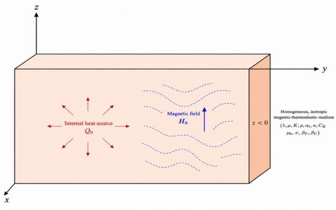
To demonstrate the analytical procedure discussed previously, we provide a numerical example accompanied by computational results. These results are analyzed within the context of the refined Lord-Shulman framework (RLS). The study focuses on examining the influence of factors such as the magnetic field, reference temperature, vertical distance, and an internal heat source on wave propagation in a thermoelastic solid. The properties of material required in numerical calculations are provided by applying the copper material constants such as Allehaibi and Zenkour38.
$$\begin{gathered} \lambda_{1} = 7.76{\mkern 1mu} x10^{9} {\mkern 1mu} N{\mkern 1mu} .{\mkern 1mu} m^{ – 2} ,{\mkern 1mu} {\mkern 1mu} {\mkern 1mu} \mu_{1} = 3.86{\mkern 1mu} x10^{9} {\mkern 1mu} N{\mkern 1mu} .{\mkern 1mu} m^{ – 2} ,{\mkern 1mu} {\mkern 1mu} {\mkern 1mu} \rho = 8954{\mkern 1mu} kg{\mkern 1mu} .{\mkern 1mu} m^{ – 3} ,{\mkern 1mu} {\mkern 1mu} {\mkern 1mu} {\mkern 1mu} C_{E} = 383.1{\mkern 1mu} {\mkern 1mu} J{\mkern 1mu} .kg^{ – 1} .{\mkern 1mu} K^{ – 1} {\mkern 1mu} ,{\mkern 1mu} {\mkern 1mu} {\mkern 1mu} {\mkern 1mu} f_{1} {\mkern 1mu} = 1,{\mkern 1mu} {\mkern 1mu} {\mkern 1mu} {\mkern 1mu} {\mkern 1mu} {\mkern 1mu} {\mkern 1mu} f_{2} {\mkern 1mu} = 2,{\mkern 1mu} {\mkern 1mu} {\mkern 1mu} {\mkern 1mu} {\mkern 1mu} {\mkern 1mu} {\mkern 1mu} G = 1, \hfill \\ \tau = 0.9{\mkern 1mu} s,{\mkern 1mu} {\mkern 1mu} {\mkern 1mu} {\mkern 1mu} \alpha_{t} = 2.78{\mkern 1mu} {\mkern 1mu} x{\mkern 1mu} 10^{ – 4} {\mkern 1mu} K^{ – 1} ,{\mkern 1mu} {\mkern 1mu} {\mkern 1mu} {\mkern 1mu} K = 386{\mkern 1mu} w{\mkern 1mu} .{\mkern 1mu} m^{ – 1} .{\mkern 1mu} K^{ – 1} ,{\mkern 1mu} {\mkern 1mu} {\mkern 1mu} T_{0} = 293{\mkern 1mu} K,{\mkern 1mu} {\mkern 1mu} {\mkern 1mu} {\mkern 1mu} {\mkern 1mu} \mu_{0} = 1.7,{\mkern 1mu} {\mkern 1mu} {\mkern 1mu} {\mkern 1mu} \varepsilon_{0} = 0.3,{\mkern 1mu} {\mkern 1mu} {\mkern 1mu} {\mkern 1mu} {\mkern 1mu} M = M_{0} + i\xi ,{\mkern 1mu} {\mkern 1mu} {\mkern 1mu} {\mkern 1mu} M_{0} = – {\mkern 1mu} 0.7,{\mkern 1mu} {\mkern 1mu} {\mkern 1mu} {\mkern 1mu} \xi = – 1, \hfill \\ t = 0.1{\mkern 1mu} s,{\mkern 1mu} {\mkern 1mu} {\mkern 1mu} V_{0} = 5{\mkern 1mu} x \, 10^{ – 9} {\mkern 1mu} m \cdot s^{ – 1} \hfill \\ \end{gathered}$$
The displacement components \(u_{1} ,\,u_{2} ,\) the thermal temperature \(\theta ,\) the stress components \(\sigma_{xx} ,\,\,\,\sigma_{xy}\), the induced magnetic field \(h,\) and the dilatation \(e,\) with respect to distance \(x\) were analyzed. These analyzes incorporated the designated value for \(y = 5.5\) during the calculation process.
Figures 2, 3, 4, 5, 6, 7, 8 highlight the differences between the displacement components \(u_{1} ,\,u_{2}\), the thermal temperature \(\theta\), the stress tensor components \(\sigma_{xx} ,\,\,\sigma_{xy}\), the induced magnetic field \(h,\) and the dilatation \(e\) for several values of the magnetic field with the reference temperature \((\,\theta_{0} = 0.09\,)\) without the internal heat source \((\,Q_{0} = 0.0\,)\). Figure 2 reveals the horizontal displacement pattern \(u_{1}\) parameterized by the distance into the medium designated x under the modifying effect of different magnetic field values. All curves begin with positive values at the surface, indicating an initial displacement response along the axis. For the curves representing lower magnetic field values, the amplitude reduces to a minimum within the spectrum \({0} \le x \le 1.6\) followed by a gradual increase and clear oscillatory behavior in the range \(1.6 \le x \le 3\) reflecting wave-like propagation. In contrast, the curves corresponding to higher magnetic field values show a rapid initial increase to a maximum at x = 2.4, then a gradual decrease to a minimum up to x = 1.6 with sustained oscillatory behavior. These findings confirm the significant influence exerted by magnetic field intensity on the nature of mechanical wave propagation within the medium. Figure 3 exhibits the vertical displacement component \(u_{2}\) in defiance of the horizontal distance in response to varying magnetic field intensities. The curves demonstrate that an increase of the magnetic field strength induces a substantial reduction in the oscillation magnitude of the vertical displacement, highlighted attributable to the magnetic field role in suppressing the mechanical motion of the medium. All profiles exhibit an oscillatory behavior that gradually decays as the distance increases, confirming the wavy nature of propagation with finite speed in accordance with generalized thermoelasticity theory. This behavior is attributed to the magnetically induced body force linked to the magneto-dynamic response of the induced currents within the medium. These findings are consistent with the theoretical assumptions of the generalized Lord-Shulman theory in describing coupled thermal-elastic-magnetic phenomena. It is clear from Fig. 4 that the thermal temperature \(\theta\) begins from positive values and obeys boundary conditions. It depicts the distribution of thermal temperature \(\theta\) against the horizontal distance x acted upon by different magnetic field intensities. All curves exhibit an oscillatory pattern that begins with positive values, followed by alternating periods of increase and decrease as x increases. Periods of sharp increase are observed near the surface (at small x), succeeded by gradual decrease phases until the field stabilizes to zero at larger x. Increasing the magnetic field strength significantly reduces the amplitude of thermal oscillations. This behavior confirms the wave-type, finite-speed heat transfer according to the extended Lord-Shulman model and demonstrates that the thermal field is confined within a limited spatial region before gradually decaying. A negative value of the temperature variation θ does not mean that the material is absorbing a “negative temperature.” Here, θ denotes the temperature change (temperature increment) relative to the reference temperature, rather than the absolute temperature. Therefore, θ < 0 simply indicates that the local temperature is lower than the chosen reference temperature. It represents a local cooling or temperature reduction, not a physically negative absolute temperature. Figure 5 depicts the behavior of the stress component values \(\sigma_{xx}\) relative to the horizontal linear coordinate x under the implications of different magnetic field intensities. \(\sigma_{xx}\) starts from negative values and obeys boundary conditions. The curves exhibit a reciprocating action starting with a maximum (negative) value at the surface x = 0, followed by alternating periods of increase and decrease as x increases. A sharp increase period is observed in the range \({0} \le x \le 1.7\) approximately, succeeded by a decrease period until x = 2.8, then a slight increase again before gradually decaying and converging to zero at a larger x. Increasing the magnetic field strength significantly reduces the amplitude of stress oscillations, which predicts wave propagation at finite speed and gradual decay with distance, confirming that all material conditions remain confined within a specific spatial district before reaching equilibrium. Figure 6 displays how the specific stress component \(\sigma_{xy}\) is distributed next to the horizontal distance x under the tradition of different magnetic field intensities. \(\sigma_{xy}\) starts from a zero value and obeys boundary conditions. All curves start null at the boundary x = 0, satisfying the constraint, and then exhibit an oscillatory pattern alternating between periods of increase and decrease as x increases. A sharp increase in stress is observed bounded by \({0} \le x \le 1.1\) reaching the greatest positive number, followed by a gradual decrease until x = 1.9 to reach a minimum negative value, then a second enhances the coverage \(2.1 \le x \le 4\)before completely decaying and approaching zero. Increasing the magnetic region strength significantly attenuates the amplitude of oscillations, confirming the role of magnetic forces in damping shear stresses. This behavior reflects the coupled wave nature of thermal, elastic, and magnetic interactions according to the extended Lord-Shulman model. The same behavior that has been observed in the literature, by Salah et al39. Figure 7 exhibits the magnitude distribution of the induced magnetic field \(h\) against the distance x owing to different magnetic field intensities. All curves with negative origins at the surface x = 0 and exhibit a clear oscillatory pattern alternating between periods of increase and decrease. A sharp increase with respect to the induced field is exhibited about \({0} \le x \le 0.8\) reaching the upper limit, followed by a sharp decrease about \({0}{\text{.8}} \le x \le 1.6\) to reach a minimum negative value, then a secondary increased dispersion \(1.6 \le x \le 2.8\) with a subsequent downward trend until approaching zero at large x. Increasing primary magnetic field strength significantly curtails the strength of the oscillation, reflecting the damping effect of the Lorentz force on induced magnetic waves. This behavior confirms the coupled wave nature of magnetic, thermal, and elastic interactions according to the extended Lord-Shulman model. The negative value of the induced magnetic field h does not indicate a negative magnetic-field magnitude. Rather, it represents the opposite direction of the induced magnetic field relative to the positive direction selected in the mathematical formulation. Such a sign reversal can arise from the magnetoelastic coupling and the interaction between the applied magnetic field, mechanical deformation, and induced electromagnetic response. Figure 8 depicts the distribution of dilatation (volumetric strain) \(e\) versus horizontal distance x under the dependence on different magnetic influence intensities. All curves start with positive values at the surface x = 0, then record a sharp decrease period about \({0} \le x \le 0.3\) reaching a minimum (negative) value, followed by a gradual increase period within the span of \({0}{\text{.3}} \le x \le 1.9\) reaching a local maximum, then a secondary contracts the interval \(1.9 \le x \le 2.9\) followed by slight oscillations before completely decaying and converging to zero at \(x \ge 4.3\). Increasing the magnetic field strength significantly reduces the oscillation amplitude. This behavior aligns with the extended Lord-Shulman (L-S) model, which predicts coupled mechanical-thermal-magnetic wave propagation at finite speed and gradual decay until reaching equilibrium.
Fig. 2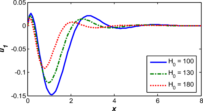
Horizontal displacement dispersion \(u_{1}\) for several values of a magnetic field.
Fig. 3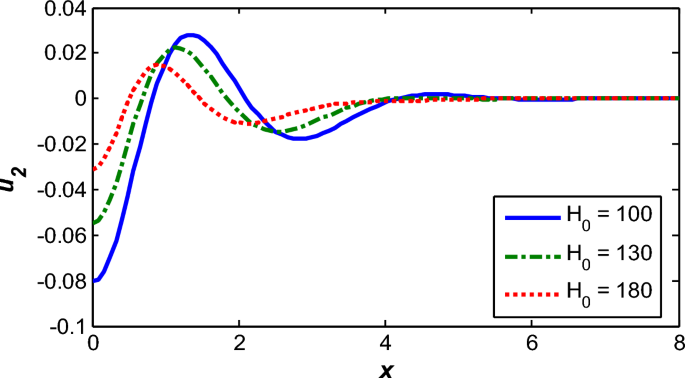
Vertical displacement dispersion \(u_{2}\) for several values of a magnetic field.
Fig. 4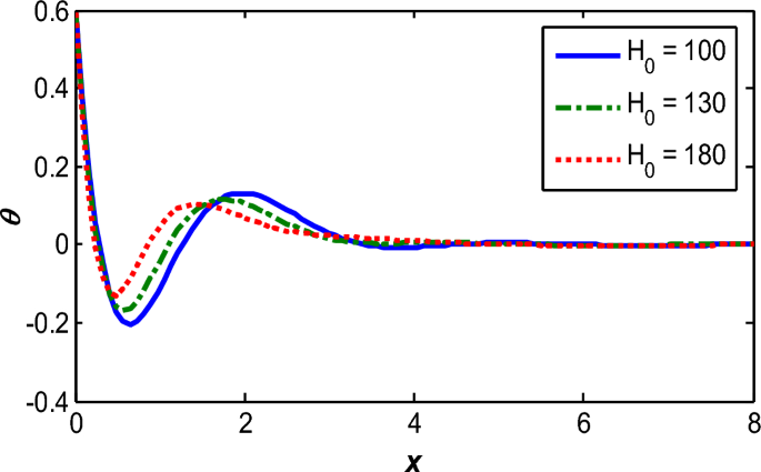
Thermal temperature dispersion \(\theta\) for several values of a magnetic field.
Fig. 5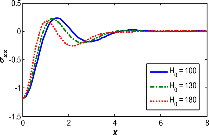
Dispersion of stress component \(\sigma_{xx}\) for various values of a magnetic field.
Fig. 6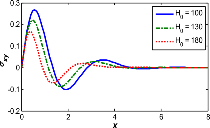
Dispersion of stress component \(\sigma_{xy}\) for several values of a magnetic field.
Fig. 7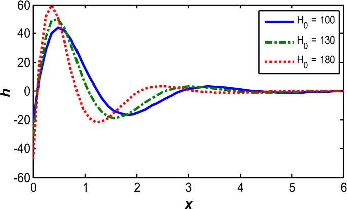
Dispersion of an induced magnetic field \(h\) for several values of a magnetic field.
Fig. 8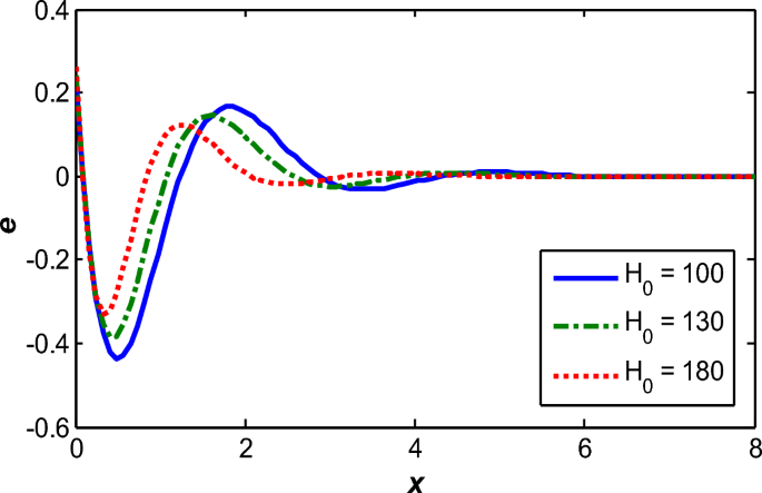
Dispersion of dilatation \(e\) for several values of a magnetic field.
Figures 9, 10, 11, 12 show comparisons between the displacement component \(u_{1} \,,\) the thermal temperature \(\theta \,,\) the stress component \(\sigma_{xx} \,,\) and the induction magnetic field \(h\) without the heat source \((\,Q_{0} = 0.0\,)\) and the magnetic influence \((\,H_{0} = 100\,)\) for different values of a reference temperature \((\,\theta_{0} = \,0.09,0.05,0.03)\). Figure 9 depicts the horizontal displacement distribution \(u_{1}\) against the distance x under the influence of different reference temperature values \(\theta_{0}\). All curves start with positive values at the surface x = 0 then record a sharp decrease about \(0.1 \le x \le 1.3\) reaching a minimum, followed by a gradual dilation of the range \(1.3 \le x \le 2.8\) reaching a local maximum, then a secondary damping of the range \(3.1 \le x \le 3.9\) before completely decaying and converging to zero. Increasing the reference temperature significantly reduces the displacement amplitude, reflecting the temperature-dependent mechanical properties through the function \(f(\theta_{0} ) = (1 – \theta_{0} T_{0} )\) where higher \(\theta_{0}\) effectively reduces the material’s elastic modulus. Figure 10 illustrates the distribution of thermal temperature \(\theta\) within a thermoelastic medium affected by different reference temperature values \(\theta_{0}\). The curves exhibit an oscillatory behavior starting from the material’s surface and gradually decaying with distance, reflecting the finite-speed wave-like nature of heat transfer according to generalized thermoelasticity models. It is evident that increasing the reference temperature reduces the amplitude of the thermal distribution, which is attributed to the thermal dependence of properties including thermal conductivity and elastic behavior modulus. Figure 11 shows the stress component \(\sigma_{xx}\) pressing on the horizontal distance x under the influence of different reference temperature values \(\theta_{0}\). All curves start with negative values at the surface x = 0, then record a sharp increase period in the set of values \({0} \le x \le 1.8\) reaching a local maximum (less negative), followed by a gradual decrease period in the range \(1.8 \le x \le 2.8,\) until reaching a local minimum, then a secondary increase period in the range \(2.8 \le x \le 4.1\) followed by slight oscillations before completely decaying and converging to zero at \(5.1 \le x\). Figure 12 illustrates the distribution of the induction magnetic field \(h\) against the horizontal distance x under the influence of different reference temperature values \(\theta_{0}\). All curves start with negative values at the surface, then exhibit an oscillatory behavior that gradually decays with distance until completely vanishing, reflecting the finite-speed wave nature of coupled interactions. Increasing the reference temperature significantly reduces the amplitude of the induced magnetic field, satisfying physically interpreted as the consequence of temperature-dependent mechanical attributes (elastic modulus) higher \(\theta_{0}\) softens the material. This behavior aligns with the refined Lord-Shulman (RLS) model, which incorporates the reference temperature effect into the coupled constitutive equations, confirming its fundamental role in modifying all physical fields.
Fig. 9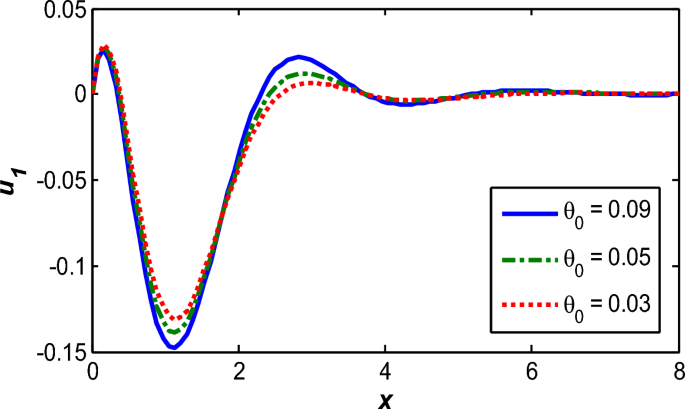
Horizontal displacement dispersion \(u_{1}\) for several values of a reference temperature.
Fig. 10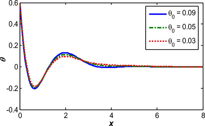
Thermal temperature dispersion \(\theta\) for several values of a reference temperature.
Fig. 11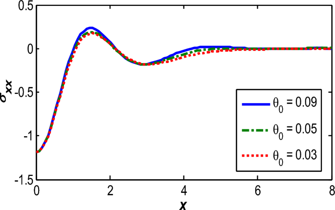
Dispersion of stress component \(\sigma_{xx}\) for several values of a reference temperature.
Fig. 12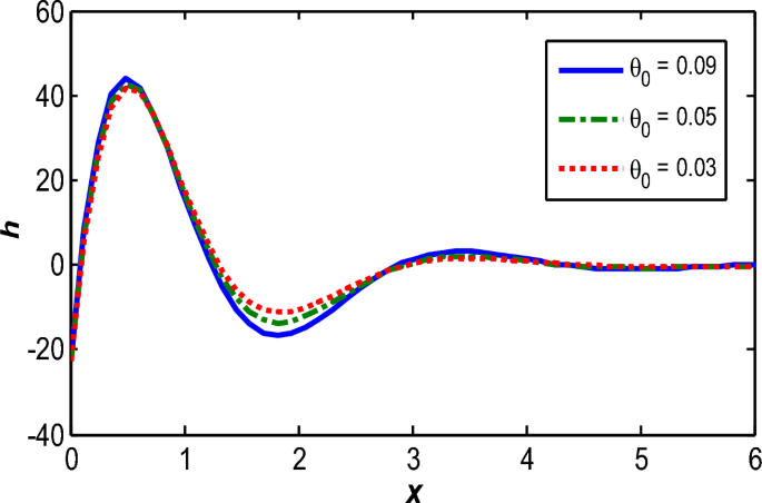
Dispersion of an induced magnetic field \(h\) for several values of a reference temperature.
Figures 13, 14, 15 analyze the interplay of the interdependence of the displacement component \(u_{2} ,\) the thermal temperature \(\theta\), and the stress component \(\sigma_{xx}\) with the reference temperature \((\,\theta_{0} = 0.09\,)\) and the region of magnetic influence \((\,H_{0} = 100)\) under different internal heat source intensities \((Q_{0} = \,0,0.0002,0.0004)\). Figure 13 depicts the distribution of vertical displacement \(u_{2}\) as a result of the distance x for several settings emanating from the internal heat source. The curves show a increase in displacement values (in the negative direction) from x = 0 to x = 1.8, reaching minimum peaks (maximum negative values at x = 2.6). After this point, the displacement begins to gradually increase with increasing xuntil approaching zero. Unsurprisingly, increasing the intensity of the thermal perturbation raises the amplitude of the negative displacement, confirming the modifying the dependence on the internal heat source on the vertical mechanical wave progression inside the medium. The same behavior that has been observed in the literature, by Othman et al40. Figure 14 charts the thermal temperature distribution θ based on different values of the internal thermal disturbance \(Q_{0}\). The curves show that temperature increases significantly with the intensity of the internal heat source, with the highest curve recorded at \(Q_{0} = \,0.0004\). All curves exhibit a continuously decreasing behavior as the horizontal distance x increases, starting with maximum values near initiating at the surface and steadily advancing, diminishing to approach zero further detached from the heat source, reflecting the cooling effect and thermal equilibrium within the medium. Figure 15 illustrates the distribution of the normal stress component \(\sigma_{xx}\) under the influence of different internal heat source conditions \(Q_{0}\). Physically, these stresses reflect the response of the thermoelastic medium to temperature changes generated by the internal heat source, where an increase in the source intensity leads to greater thermal expansion, thereby generating internal stresses due to the resistance of elastic fibers to expansion. In both figures, stress values peak in the immediate vicinity of x = 0 and then gradually decrease with distance from the origin, indicating that thermal and mechanical effects diminish away from the source. Increasing \(Q_{0}\) significantly raises the stress values, confirming the pivotal way in which the internal heat source influences the stress field within the medium.
Fig. 13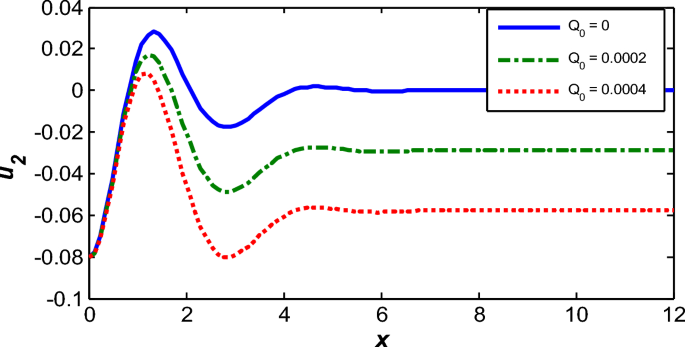
Vertical displacement dispersion \(u_{2}\) for several values of an internal heat source.
Fig. 14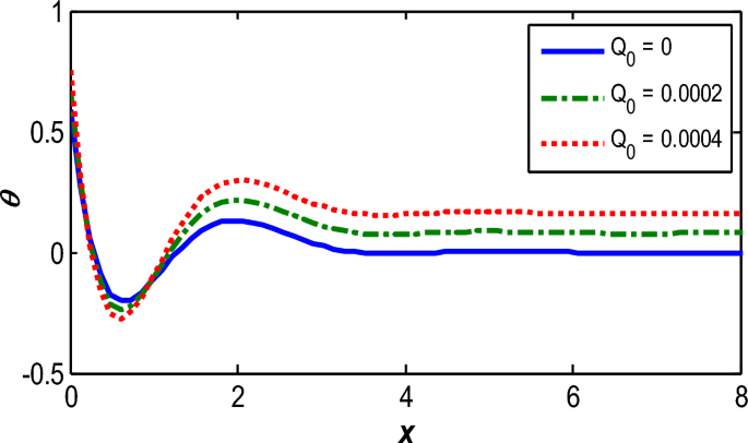
Thermal temperature dispersion \(\theta\) for several values of an internal heat source.
Fig. 15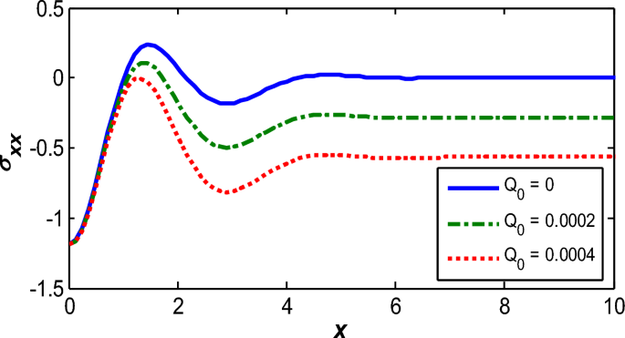
Dispersion of stress component \(\sigma_{xx}\) for several values of an internal heat source.
Figures 16–18 show the three-dimensional distribution, whereas, Fig. 16 depicts the three-dimensional distribution of temperature \(\theta\) where the highest values are concentrated at the heat source at small x and gradually decrease with increasing spatial dimensions (x, y) reflecting the dissipative nature of thermal waves and confirming the role of thermal conduction in energy dissipation. Figure 17 illustrates the induced magnetic field \(h\) exhibiting similar how the system behaves under magneto-thermal coupling; deformations resulting from thermal stresses generate a magnetic field that peaks surface-localized and fades outward. Figure 18 displays the distribution of dilatation \(e\) (relative volume change), which reflects the medium’s response to thermal and magnetic stresses, with high dilatation values concentrated near the heat source and gradually diminishing away from it. Together, these figures highlight the coupled nature of thermal, elastic, and magnetic fields, confirming that all physical variables are significantly influenced by the internal heat source and magnetic field, with consistent dissipative behavior that aligns with the theoretical assumptions of the refined Lord-Shulman (RLS) framework.
Fig. 16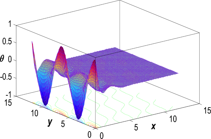
Dispersion of thermal temperature \(\theta\) in the 3D via refined L-S framework.
Fig. 17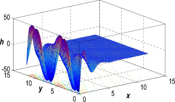
an induced magnetic field \(h\) in the 3D via refined L-S framework.
Fig. 18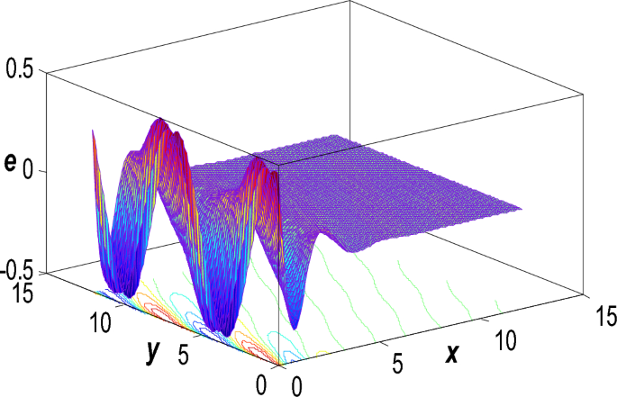
Dispersion of dilatation \(e\) in the 3D via refined L-S framework.