
Airy beam generation and characterization
To model the best Airy beam for delivering data to an obstructed user, we first look into the field distribution of an Airy beam. Consider a sub-THz wireless transmitter (e.g., a base station) with an aperture along the x direction transmitting an Airy beam with the propagation direction along z. We can write the field distribution of this 1D finite-energy Airy beam as33,52:
$$E\left(x,z\right)={{{\rm{Ai}}}}\left(\frac{x}{{x}_{o}}-\frac{{z}^{2}}{4{k}^{2}{x}_{o}^{4}}+i\frac{\alpha z}{k{x}_{o}^{2}}\right){e}^{i\frac{z}{2k{x}_{o}^{2}}\,\left(\frac{x}{{x}_{o}}\,-\,\frac{{z}^{2}}{6{k}^{2}{x}_{o}^{4}}\,+\,{\alpha }^{2}\right)}{e}^{\frac{\alpha }{{x}_{o}}\left(x-\frac{{z}^{2}}{2{k}^{2}{x}_{o}^{3}}\right)},$$
(1)
where \({{{\rm{Ai}}}}(\cdot )\) is the Airy function. The truncation parameter \(\alpha\) ensures the physical realization of Airy beams with finite energy, \({x}_{o}\) is a transverse scale that controls the curvature of the resulting beam, and \(k\) is the wavenumber. Under ideal infinite-power Airy beams (generated with infinitely large apertures) where \(\alpha=0\), a propagating trajectory of \(x\left(z\right)=\frac{{z}^{2}}{4{k}^{2}{x}_{o}^{3}}\) can be retrieved by setting the argument of the Airy function to 0. The parabolic trajectory can be tuned by varying parameter \({x}_{o}\), and its finite-energy radiation pattern can be generated by exciting the transmitting aperture with \(E\left(x,\,0\right)={{{\rm{Ai}}}}\left(\frac{x}{{x}_{o}}\right){e}^{\frac{\alpha x}{{x}_{o}}},\) as shown in Fig. 1a.
Fig. 1: Generation and features of Airy beams.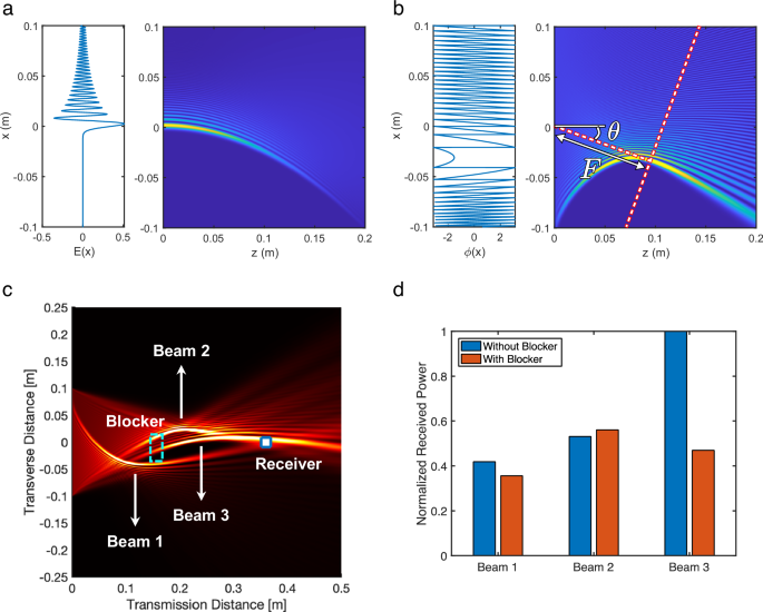
a A self-healing finite-energy Airy beam can be generated by applying an electric field described by a scaled Airy function at the transmitting aperture, along with a truncation factor. The radiation pattern is calculated by the theoretical closed-form Airy beam propagation equation with \(\alpha\) = 0.05. Here, we set \({x}_{o}\) = 2.5 mm at 120 GHz. b A desired arbitrary Airy beam can be generated at a specified distance and orientation using Fourier optics. A cubic phase and a focusing phase mask are superpositioned at the transmitting aperture to create an Airy profile at the marked plane, from which onward the Airy beam propagates. The red dashed line shows where the Airy propagation starts. Here, we set \(B=7,{F}=0.1{m},\,\theta=-{20}^{\circ }\) at 120 GHz. c There exists an infinite number of feasible Airy trajectories that can be configured between the transmitter to the receiver. Here, we show 3 examples of such beams. d The received power of the 3 example beam configurations with and without the blocker.
Despite controllable curvature, the resulting wavefront has a limited ability to curve around arbitrary obstacles. This is because the self-acceleration and curving start immediately from \(z=0\), independent of the obstruction’s location or the receiver’s position. To address such limitations, we adopt principles from Fourier optics to enforce self-acceleration at a desired point in space, which can then be adapted based on the geometric properties of the wireless medium (e.g., blocker location and size, as well as the receiver’s location). Specifically, an Airy profile can be synthesized in the Fourier plane by imposing a cubic phase at the transmitting plane30,38:
$$\phi (x,0)=\frac{1}{3}{\left(2\pi B\right)}^{3}{x}^{3}-\frac{2\pi }{\lambda }\sqrt{{\left(F\sin \theta -x\right)}^{2}+{\left(F\cos \theta \right)}^{2}},$$
(2)
where \(\phi \left(x,0\right)\) is the phase profile used at the transmitter (\(z=0\)), \(F\) is the focal length, \(\theta\) represents the steering angle, \(B\) is the curvature coefficient in the cubic phase, and \(\lambda\) is the wavelength. The resulting wave propagation creates a curved beam with self-acceleration starting at a rotated plane, crossing \(({{x}_{F},{z}}_{F})=(F \sin \theta,\,F \cos \theta)\). An example can be seen in Fig. 1b, in which an Airy profile is projected at focal distance \(F=0.1\) m and \(\theta={-20}^{\circ }\) (the red dashed line shows where the Airy propagation starts). The field propagation is calculated by solving the Rayleigh–Sommerfeld integral using Fast Fourier Transform (FFT).
Under such parameterization, a curved Airy wavefront can be uniquely represented by a combination of \(\left(B,F,\theta \right)\), which describe curvature, focal length, and steering angle, respectively. Indeed, the space of finite-energy Airy beams can be characterized by these three parameters (see Supplementary Note 1). Comparing Fig. 1b with Fig. 1a, we observe that Airy beam generation based on Fourier optics is promising for blockage mitigation in practical sub-THz wireless networks because (i) antenna arrays with phase-control only are sufficient to generate desired beams (i.e., no need for amplitude control per antenna), which complies with commonly available analog phased arrays53,54 and (ii) the trajectory can be adjusted with additional flexibility to the geometric specification of the wireless medium.
Max-power trajectory shaping
Exploiting the Airy near-field wavefront in practice demands fundamental changes in several aspects of wireless networking. In today’s wireless networks operating in mmWave bands, the transmitter has to align its directional beam toward the location of the receiver. Instead, here, a curved trajectory should be established between the transmitter and the receiver while taking into consideration the potential obstructions. Geometrically, an infinite number of trajectories can be engineered. Figure 1c depicts a few examples of such paths for a simple setting. Hence, merely finding a trajectory that satisfies the geometric requirements alone is not sufficient; it is, instead, important to find the optimal Airy beam that delivers maximum power to the receiver under a given wireless environment. Figure 1d shows that different curved trajectories between the transmitter and receiver may offer vastly different power levels, with and without obstruction.
Such link budget analysis and power calculation are straightforward in far-field situations and are governed by the well-known Friis equation (see Supplementary Note 2). However, capturing the received power in the near-field is much more complicated and requires calculating the radiated field based on the Rayleigh–Sommerfeld integral:
$$E\left(x^{\prime},y^{\prime},z^{\prime}|{E}_{{tx}}\right)=\frac{1}{2\pi }\int \int {E}_{{tx}}\left(x,y,0\right)\left[\frac{{{z}^{{\prime} }e}^{{ikr}}}{{r}^{2}}\,\left(\frac{1}{r}-{ik}\right)\right]d{A}_{{tx}},$$
(3)
where \({E}_{{tx}}\left(x,y,0\right)\) represents the initial E-field at the transmitter (configured to create a particular trajectory), k is the wavenumber, \(r=\sqrt{{\left({x}^{{\prime} }-x\right)}^{2}+{\left({y}^{{\prime} }-y\right)}^{2}+{{z}^{{\prime} }}^{2}}\) is the point-wise distance between each element on the transmitter to the near-field point-of-interest, and the integral is performed over the transmitter aperture \({A}_{{tx}}\). We note that the field calculation in Eq. (3) does not have a closed-form solution for Airy beams generated through Fourier optics and should be solved numerically. More importantly, when the environment is inhomogeneous (e.g., under the presence of blockers), Eq. (3) cannot be calculated in one shot; instead, it must be solved iteratively with small step sizes along the propagation direction z (details are provided in Supplementary Note 3). Based on the iteratively calculated electric fields, for any given Airy profile, we can write the delivered power as follows:
$${P}_{{rx}}=\int \int {\left|E\left({x}^{{\prime} },{y}^{{\prime} },{z}^{{\prime} }|{E}_{{tx}}\right)\right|}^{2}\,d{A}_{{rx}},$$
(4)
where \(E\left({x}^{{\prime} },{y}^{{\prime} },{z}^{{\prime} }|{E}_{{tx}}\right)\) is the radiation pattern conditioned on the initial transmitted fields, as calculated in Eq. (3). \({P}_{{rx}}\) is the received power, and the integral is performed over the receiver aperture.
Building on top of Eqs. (3) and (4), one can in principle find the best Airy trajectory delivering the maximum link budget by solving the following optimization framework for a given wireless environment, through iteratively searching over theoretically feasible Airy beams (conventional gradient-based optimization methods cannot be applied since the objective function yields no closed-form expression or gradient):
$$\left({B}^{\star },{F}^{\star },{\theta }^{\star }\right)={{{{\rm{argmax}}}}}_{\left(B,F,\theta \right)}\int \int {\left|E\left({x}^{{\prime} },{y}^{{\prime} },{z}^{{\prime} }|{E}_{{tx}}\right)\right|}^{2}\,d{A}_{{rx}},$$
(5)
where \(\left({B}^{\star },{F}^{\star },{\theta }^{\star }\right)\) are the optimum Airy beam parameters. Unfortunately, exhaustively solving Eq. (5) is not feasible in practice due to the massive parameter space (infinite in principle) and the significant computational cost of numerical field distribution calculations (iterative Rayleigh–Sommerfeld integral). Further, this optimization has to be repeated frequently in dynamic environments as the solution is very sensitive to the real-time location of the receiver and the blocker. In other words, not only is a brute force measurement of all possible Airy beams not feasible (due to prohibitively large time overhead), but even computing the delivered power under a single specific Airy beam configuration incurs significant computational cost. Consequently, evolutionary algorithms also incur prohibitively slow and sub-linear convergence rates (especially in continuous search spaces) that are significantly impacted by the complexity of the problem51,55 and the absence of a closed-form equation for the objective function shown in Eqs. (3)–(5). Specifically, each evolution step would require thousands of iterations when solving the integral in Eq. (3), which takes second-scale computation time even with high-performance PCs/servers (see Supplementary Note 3). We note that such overheads make evolutions particularly time-prohibitive for wireless communication scenarios with limited budget in both time and computational resources. In contrast, we introduce a data-driven approach to optimize Airy beam shape with zero-shot execution, where complexity and overheads are offloaded to the pre-training stage.
Airy trajectory learning
We exploit physics-driven insights to train a supervised neural network that solves Eq. (5) for the optimal Airy configuration. First, we use ray optics to define a blockage percentage (bl) that captures the ratio of blocked rays to the total emitted rays from the transmitter. This blockage parameter, which is purely a geometric feature, plays an important role in the potential link budget gain achieved by a curving beam, i.e., the gain offered by Airy beams (relative to a conventional focused beam) grows as \({bl}\) increases. For the same reason, exploiting Airy self-accelerating beams can significantly reduce the shadow area of an obstruction (see Supplementary Note 4). Accordingly, we use \({bl}\) to threshold the activation of our neural network (i.e., reverting to conventional focused beams when the LOS path remains unblocked). Further, based on its relationship (though complicated as shown in Supplementary Note 4) to optimal trajectories, we also exploit bl as a direct input feature to the neural network that impacts its convergence to the optimal Airy parameters.
Second, based on the physics of Airy beam generation, we know that a negative curvature coefficient (\(B < 0\) in Eq. (2)) results in an upward trajectory and vice versa. Further, ray optics suggests that if the receiver is located below the line connecting the center of the transmitter array and obstacle, then geometrically, an Airy beam that curved around the lower side of the obstacle with an upward trajectory is more likely (\({B}^{\star } < 0\) in Eq. (5)). We call this type of environmental setting “convex” topologies as they likely result in upward curved beams, and we call other settings “concave” topologies due to similar reasons (details explained in Supplementary Note 5). Intuitively, according to Fourier optics and ray optics principles, we can show that for each “convex” topology with optimal beam solution \(({B}^{\star },{F}^{\star },{\theta }^{\star })\), there exists an equivalent mirrored environmental setting with “concave” topology where the optimal Airy beam parameters are \(({-B}^{\star },{F}^{\star },{-\theta }^{\star })\), and vice versa. Hence, we can improve the neural-network convergence and accuracy by making it learn how to configure optimal beams for only one type of topology, applying appropriate geometric mirroring at the input and parameter sign flipping at the output (\({B}^{\star }\to -{B}^{\star }\), \({\theta }^{\star }\to -{\theta }^{\star }\)) to generalize to all settings. To streamline the flipping process and facilitate convergence, we define \(\Delta x={x}_{{RX}}-{x}_{{obs}}\) as an additional input feature to the neural network, where \({x}_{{RX}}\) and \({x}_{{obs}}\) represent the center of the receiver and obstruction in the \(x\) -plane, respectively (Supplementary Note 5). Finally, for a given transmitter aperture Atx and frequency f, only a certain range of Airy parameters \(\left(B,F,\theta \right)\) result in effective curving trajectories based on near-field electromagnetics. Hence, we rely on the understanding of near-field wave propagation and Airy beam generation to refine the search space for true optimal Airy parameter labels during data collection for a given aperture size and frequency (see Supplementary Note 6).
Figure 2a illustrates the high-level description of our framework that aims to enable blockage mitigation by adaptively learning the best self-accelerating Airy beam in dynamic sub-THz wireless networks. Figure 2b depicts the architecture of trajectory learning with geometric environment inputs (e.g., locations of the receiver and the blocker) and physics-inspired features (bl and \(\Delta x\)). The detail of the neural network is provided in Supplementary Note 7. Figure 2c shows the normalized power delivery performance of AI-adapted Airy beams compared to steered beams, focused beams, and brute force optimal Airy beams across 400 simulated test environments. Particularly, the AI-based beam shaping framework can successfully learn the optimal Airy beam and deliver the same amount of power (less than 0.5 dB difference on average) to the receiver compared with a brute force Airy beam optimization. Further, curved trajectories can realize a significant power gain compared with conventional far-field Gaussian beam steering (more than 17.7 dB on average) and near-field beam focusing (more than 3.4 dB on average), highlighting the potential of Airy beams for blockage mitigation. While this result is achieved in 2D settings, similar principles can be extended to learning curved beams in more complicated 3D environments with multiple obstructions, as illustrated in Supplementary Note 8. We note that although a 2D circular Airy beam56 in principle also shows self-healing properties, we stay with 2D rectangular Airy beams in our 3D environment model for the compatibility with our optimization framework as well as efficient energy confinement. Finally, the learning framework in Fig. 2 assumes that minimal knowledge of the environment is available, merely including the location of the receiver, the location of the blocker, and its size. Just like in the case of beam focusing that requires the receiver location information, some form of sensing input (e.g., using cameras, lidars, radar) is required at the transmitter to acquire geometric information about the environment (implementing such sensing techniques is beyond the scope of this work). We explore the sensitivity of near-field Airy beam shaping to such localization uncertainties in Supplementary Note 9.
Fig. 2: Illustration of the physics-informed learning framework for optimal Airy beams.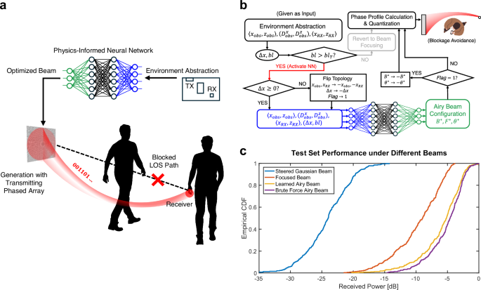
a An optimal self-accelerating beam is learned that can successfully curve around the LOS obstruction and deliver maximum power to the receiver. b The schematic of our learning-based beam shaping framework, in which the NN-based Airy optimization is only activated when there is LOS blockage, i.e., when blockage parameter \({bl}\) exceeds a pre-defined threshold \(b{l}_{T}\). c The empirical CDF of normalized received power across 400 different simulated test scenarios (with \({bl} > 80\%\)). The learned Airy beam achieves similar power to the optimal Airy beam found via the brute force scheme. Further, the boost in received power is substantial compared with the steered Gaussian beam and the focused beam.
Experimental realization
We implement AI-learned self-accelerating Airy beams with over-the-air experiments in the D-band regime. We use a pre-trained neural network to learn the optimal Airy configuration for unseen experimental configurations. We emphasize that this approach requires a one-time training overhead, but the time and computational overhead of predicting the best Airy beam with a pre-trained neural network is minimal, opening the possibility for adoption in practical mobile wireless networks. The details of the experimental setup are provided in the “Methods” section and Supplementary Note 10. First, Fig. 3a, b shows that the calculated Airy beam trajectories can be physically realized in the experiments. In this experiment, we transmit a single tone at 120 GHz. We note that the slight discrepancy (if any) between measured and simulated patterns could be caused by the alignment of the setup, discretization of transmitting elements (as opposed to a continuous aperture), and imperfect metasurface fabrication. Interestingly, the half-power bandwidth supported by an Airy communication link depends on the exact trajectory of the beam, which itself varies with the receiver location and the blockage conditions. Hence, distinct from conventional wireless networks, the bandwidth for Airy beam communication is location and environment dependent (see Supplementary Note 11 for theoretical derivation and analysis). The root cause of such dependency is that the Airy beam phase profile at the transmitter (derived in Eq. (5)) is optimized for the center frequency; thus, different frequencies follow slightly different curving trajectories, which leads to power reduction at the receiver location. As discussed in Supplementary Note 11, beams with sharper curvatures cause larger spectral deviation and lower bandwidth, consequently. Similarly, a larger propagation distance between the receiver and the obstruction yields lower bandwidth. Nevertheless, we demonstrate the generation of wideband curved links, where high bandwidth can be achieved up to a certain distance limit. Figure 3c shows the measured radiation heatmaps of the same example setting in Fig. 3b, but this time transmitting at 115 GHz and 125 GHz. To quantitatively analyze the bandwidth of such a curved trajectory, we extract the main trajectory from these heatmaps and use typical polynomial fitting in Fig. 3d. As shown, the trajectories slightly deviate as we move away from the center frequencies. Regardless, for a small receiver aperture size of 5 mm (4-element antenna array at 120 GHz), a large bandwidth of 10+ GHz can be realized for propagation distances up to 12 cm and 5+ GHz up to 23 cm. The ability to create a stable wave trajectory for a wide bandwidth is important, as the communication link capacity grows linearly with bandwidth. We emphasize that our neural network framework is designed to learn the optimal beam with maximum deliverable power at the center frequency. Alternatively, one could re-train the neural network to maximize the channel capacity by taking into account both received power and bandwidth.
Fig. 3: Experimental realization of Airy beams.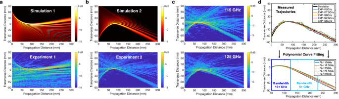
a, b We compare the measured field propagation of two example Airy beams with simulations. Airy parameters for the left and right figures are (\(B=-10,{F}=0.1 \, m,\,\theta={0}^{\circ }\)) and (\(B=7,{F}=0.08 \, m,\,\theta={0}^{\circ }\)), respectively. All figures are normalized and shown in dB scale. Measurements are at 120 GHz and indicate good agreement with simulated patterns. c The measured near-field radiation pattern does not change drastically as we deviate from the center frequency (120 GHz), suggesting that these beams can carry GHz-scale bandwidths required for establishing Gbps-scale data rates. d Measured curved trajectories stay relatively consistent across experiments from 115 GHz to 125 GHz. Bandwidths are quantified with 3-dB beamwidth, a small receiver aperture size, and polynomial-fitted curves, showing wideband trajectories especially at shorter observer distances.
Figure 4 illustrates how the Airy beam is adapted in dynamic settings: (a) with a moving obstacle; and (b) with a moving receiver. First, in Fig. 4a, an obstacle moves on a linear path and causes a transient line-of-sight blockage with the blockage percentage (bl) changing from 25% to 76% and then improving to 73% in three consecutive timestamps. At \({bl}=25\%\), the blockage setting is not severe (i.e., \({bl}\) below activation threshold) and thus the neural network is not activated, and the resulting wavefront is a focused beam (in this experiment, the threshold for activating the Airy shaping framework was assumed \(b{l}_{T}=70\%\)). At timestamps 2 and 3, a self-accelerating beam is formed curving around the obstruction as shown. Interestingly, a slight motion of the blocker between timestamps 2 and 3 results in a completely different-looking optimized Airy beam, i.e., bending from the top of the blocker vs from the bottom. We conducted a similar experiment in which the blocker remained fixed, but the receiver was linearly moving closer to the blocker (into the shadow region), as shown in Fig. 4b. As expected, the received SNR worsens under focused beam and steered beam as the blockage ratio increases. Further, the predicted Airy beam provides a meaningful SNR gain across all settings. As shown, the curvature coefficient of the optimized beam \(({B}^{\star })\) decreases, indicating a higher level of bending as blockage worsens. In each experiment, the measured field propagation matches well with the corresponding EM simulation.
Fig. 4: Performance of predicted Airy configurations in blockage mitigation.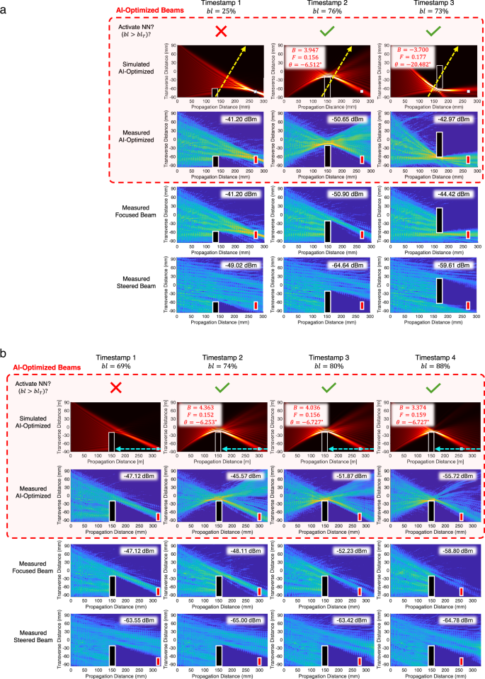
Measured near-field radiation patterns are shown for both AI-optimized beams and baseline beams. The received power is calculated by integrating over the red receiving aperture and is marked within each measurement figure. The measured wave propagations are in agreement with simulation results. Comparison with conventional Gaussian beam steering and beam focusing indicates the achieved power gain realized by the AI-optimized Airy beam. a An obstruction in the line-of-sight path moves along a linear trajectory shown with a yellow dashed line. As seen, even a slight movement of the blocker may result in a completely different prediction of the curved beam trajectory. b A receiver walks into the shadow region of an obstruction. The proposed AI framework adapts the Airy beam parameters to maximize receiver power under each setting.
Finally, the SNR enhancements offered by the neural network-predicted Airy beams are sufficient to improve the link performance and BER under LOS blockage. Figure 5a shows an illustration of our experimental setup for data transmission, in which 1 million symbols are transmitted for each BER calculation. Figure 5b shows data transmission performance under an example blockage scenario at 124 GHz with 8-QAM and 16-QAM modulations, under (i) beam focused towards the receiver and (ii) AI-predicted Airy beam. It is visually evident that, under LOS blockage, the constellation improves with the Airy beam compared with the conventional focused beam. To further quantify this result, we show in Fig. 5c the experimentally measured uncoded BER under Airy beam and focused beam for four different modulations (BPSK, 4QAM, 8QAM, 16QAM), and under several communication bandwidths, with and without LOS blockage. While the focused beam yields significantly lower BER when the LOS path is clear, as expected, our results reveal that near-field self-accelerating beams (when optimized) can outperform focused beams when the LOS path is blocked, independent of modulation or bandwidth in use. While the exact amount of BER improvement is a complicated function of environment, transmitter aperture, and physical layer parameters, indeed, orders of magnitude improvement in BER can be observed in certain configurations (e.g., more than three orders of magnitude for BPSK at 3+ GHz bandwidth).
Fig. 5: Data modulation and BER performance.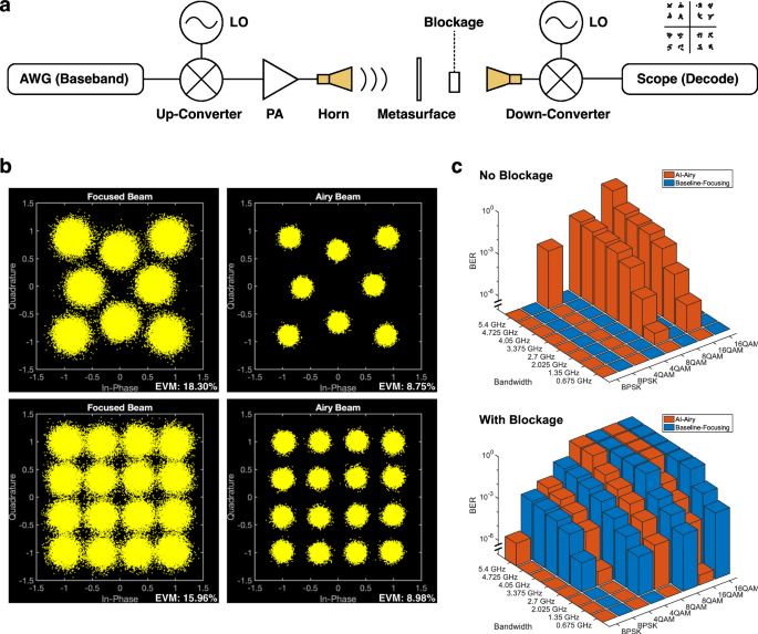
We transmit data over the air in one of the test settings and report the performance of the AI-learned Airy beam as compared to the focused beam. a Schematic flowchart illustration for data transmission experiments. b Constellation plots for 8-QAM and 16-QAM under LOS blockage, measured with a bandwidth of 700 MHz at a center frequency of 124 GHz. As marked, the optimized Airy beam achieves a significant decrease in EVM. c We compare the measured uncoded BER of the AI-learned Airy beam and the baseline focused beam under various modulation schemes and transmission bandwidths, with and without the blockage. Under LOS blockage, the measured BER is consistently and considerably lower with our Airy beam shaping framework. For instance, almost three orders of magnitude improvement can be seen under BPSK and 3+ GHz bandwidth. For comparison, we report the BER with no LOS blockage, where the focused beam outperforms our Airy optimization, as expected (i.e., no need to activate NN when there is no blockage). It is worth noting that, while LOS blockage increases BER for both beams, our AI-learned Airy beam shows significant resiliency against it, thus realizing effective blockage mitigation.