
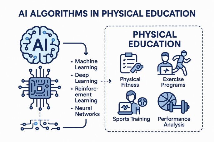
PE is essential for the development of physical fitness, motor skills, mental health, and lifelong healthy habits in students; thus, it is a pillar of holistic education in contemporary institutions. As technology continues to improve at an alarming rate, AI algorithms are becoming increasingly common in the delivery, monitoring, and personalization of PE programs. Real-time performance monitoring, customized feedback, and data-based training programs can be achieved through AI-powered systems, including pose estimation tools, adaptive training optimizers, and interactive coaching assistants, which can dramatically improve learning outcomes and engagement. Nevertheless, the large number of possible AI solutions and the trade-offs between accuracy, adaptability, ease of use, and resource demands necessitate careful and systematic DM to choose the most appropriate AI algorithms for PE requirements. A practical, uncertainty-sensitive DM framework can help educators and administrators make informed, transparent, and sensible decisions, ensuring that the chosen AI technologies support educational objectives and bring the most value to both students and institutions.
To demonstrate the feasibility and practical value of the proposed q-RLDF WASPAS framework, a real-world case study focusing on the selection of the most suitable AI algorithm for enhancing PE programs is chosen. The goal of this case study is to assist PE instructors and institutional DMKs in choosing AI solutions that best align with their objectives of improving training effectiveness, ensuring student safety, and personalizing learning experiences. To provide a balanced and credible evaluation process, three domain experts/DMK were selected based on clear criteria: practical experience in PE technology, technical expertise in AI for sports data analytics, and strategic insight into educational technology policy. Each DMK has at least 5 years of post-qualification experience. This diversity ensures the DM process reflects operational, technical, and organizational realities. Based on recent trends in AI algorithms and DMK’s opinions, five widely recognized AI algorithms \(\:{{\Lambda\:}}_{i},i=\text{1,2},\dots\:,5\) with proven applications in sports science and physical training, are considered alternatives. These alternatives represent a broad spectrum of intelligent capabilities ranging from real-time posture tracking and motion analysis to adaptive training plan generation and personalized feedback delivery. The selected widely recognized AI algorithms with a proven track record in sports science are:
\(\:{{\Lambda\:}}_{1}:\) Convolutional neural network-based motion analysis (CNN-MA),
\(\:{{\Lambda\:}}_{2}:\) Reinforcement learning based training optimizer (RL-TO),
\(\:{{\Lambda\:}}_{3}:\) Expert system for exercise prescription (ES-EP),
\(\:{{\Lambda\:}}_{4}:\) Hybrid AI tutor with natural language processing (HAI-NLP),
\(\:{{\Lambda\:}}_{5}:\) Wearable sensor data mining algorithm (WSDMA).
Following a thorough analysis of recent and relevant literature41,42,43,44,45,46,47,48, eight criteria \(\:{\mathfrak{S}}_{j},\:j\:=\:1,\:2,\:\dots\:,\:8\:\)are identified as the most significant determinants of AI algorithm performance in PE. These requirements encompass various technical, pedagogical, and practical aspects, which play a crucial role in determining the effectiveness and applicability of AI models in dynamic PE settings. They are chosen based on both empirical results and expert opinion on which attributes have a significant impact on the performance of an algorithm in a real educational context. The detail of the criteria is given below:
\(\:{\mathfrak{S}}_{1}:\) Prediction accuracy (The extent to which the algorithm accurately classifies or predicts the physical performance of students, their fitness, or their injury risk).
\(\:{\mathfrak{S}}_{2}:\) Processing time (The duration that it takes to train the AI model and process large amounts of student movement or biometric data).
\(\:{\mathfrak{S}}_{3}:\) Interpretability (How easily coaches, PE instructors, and students can understand how the algorithm makes its predictions or recommendations).
\(\:{\mathfrak{S}}_{4}:\) Resource consumption (The computational and hardware resources needed to deploy and maintain the algorithm).
\(\:{\mathfrak{S}}_{5}:\) Scalability (The capacity to process more and more students, a variety of sports activities, and bigger data without a performance decline).
\(\:{\mathfrak{S}}_{6}:\) Personalization capability (The extent to which the algorithm can be adjusted to the individual physical state of students, their goals, and progress in the long term).
\(\:{\mathfrak{S}}_{7}:\) Integration with existing modules (The ease with which the AI solution will be able to integrate with wearable devices, learning management systems, or innovative campus platforms, and existing PE software).
\(\:{\mathfrak{S}}_{8}:\) Data privacy and security (The level at which the algorithm facilitates safe data processing and adheres to the privacy requirements of sensitive health or biometric data of students).
The interrelationship between the chosen criteria, available AI algorithms, and selection of the best AI algorithm for PE is shown in Fig. 3.
Fig. 3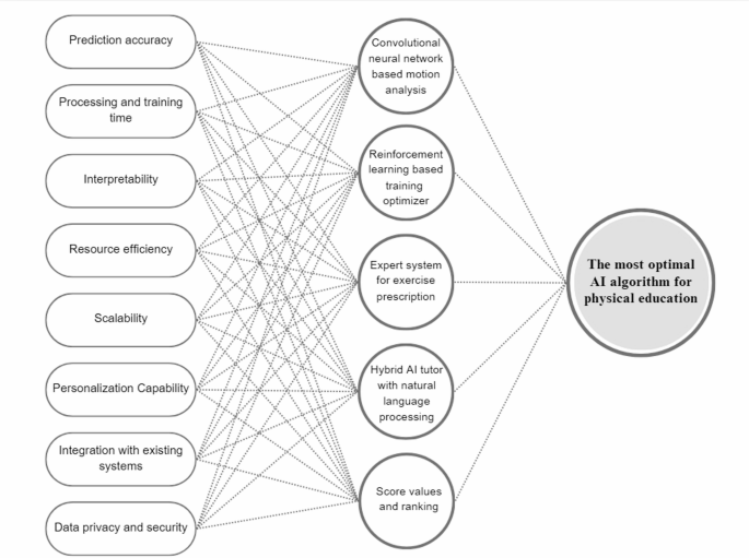
Interrelationship among criteria, available AI algorithms, and selection of the most optimal algorithm.
Step 1. In this step, each DMK was independently provided with a structured questionnaire containing eight selected evaluation criteria and five alternatives for AI algorithms. They rated the importance of each criterion and the performance of each AI algorithm against each criterion in the form q-RLDFNs. These preferences are further arranged in the form of decision matrices. The DMK’s preferences are arranged in the form of decision matrices and are given in Tables 1, 2 and 3.
Table 1 Decision matrix \(\:{M}^{\left(1\right)}\).Table 2 Decision matrix \(\:{M}^{\left(2\right)}\).Table 3 Decision matrix \(\:{M}^{\left(3\right)}\).
a)
\(\:\stackrel{-}{M}{}_{ji}=\frac{1}{\delta\:}\sum\:_{k=1}^{\delta\:}{d}_{ji}^{\left(k\right)}\), used to find group average matrix \(\:\stackrel{-}{M}=\left[\stackrel{-}{M}{}_{ji}\right]\).
b)
\(\:{\zeta\:}_{k}=\sum\:_{j=1}^{\beta\:}\sum\:_{i=1}^{\alpha\:}{\chi\:}_{q-RLDF}\left({M}_{ji}^{\left(k\right)},\stackrel{-}{M}{}_{ji}\right)\), is utilized to find the total dissimilarity matrix where \(\:{\chi\:}_{q-RLDF}\left({M}_{ji},\stackrel{-}{M}{}_{ji}\right)\) represents the distance function between two q-RLDFNs given by:
$$\:{\chi\:}_{q-RLDF}\left({M}_{ji},\stackrel{-}{M}{}_{ji}\right)=\sqrt{\frac{1}{4}\left[{\left({{\Gamma\:}}_{{M}_{ji}}-{{\Gamma\:}}_{\stackrel{-}{M}{}_{ji}}\right)}^{2}+{\left({\text{{\rm\:Y}}}_{{M}_{ji}}-{\text{{\rm\:Y}}}_{\stackrel{-}{M}{}_{ji}}\right)}^{2}+{\left({\eta\:}_{{M}_{ji}}-{\eta\:}_{\stackrel{-}{M}{}_{ji}}\right)}^{2}+{\left({\vartheta\:}_{{M}_{ji}}-{\vartheta\:}_{\stackrel{-}{M}{}_{ji}}\right)}^{2}\right]}$$
iii)
The consensus level (CL) is measured by using:
$$\:CL=1-\frac{1}{\delta\:}\sum\:_{k=1}^{\delta\:}\frac{{\zeta\:}_{k}}{{\zeta\:}_{max}}\in\:\left[\text{0,1}\right]$$
For predefined consensus threshold \(\:C{L}_{\text{t}\text{h}\text{r}\text{e}\text{s}\text{h}\text{o}\text{l}\text{d}}=0.8\), the computed \(\:CL=0.81\). Therefore, the relation \(\:CL\ge\:C{L}_{\text{t}\text{h}\text{r}\text{e}\text{s}\text{h}\text{o}\text{l}\text{d}}\) is satisfied, and consensus is met.
d)
Since there is consensus among DMK’s preferences, consensus-based weights are computed using \(\:{\psi\:}_{k}^{{\prime\:}}=\frac{\raisebox{1ex}{$1$}\!\left/\:\!\raisebox{-1ex}{${\zeta\:}_{k}$}\right.}{\sum\:_{k=1}^{\delta\:}\raisebox{1ex}{$1$}\!\left/\:\!\raisebox{-1ex}{${\zeta\:}_{k\_}$}\right.}\), where \(\:\sum\:_{k=1}^{\delta\:}{\psi\:}_{k}^{{\prime\:}}=0\).
The weights of DMKs and criteria are computed using the above relations, which ought to be \(\:{\psi\:}_{k}^{{\prime\:}}={\left\{\text{0.35,0.40,0.25}\right\}}^{T}\), and \(\:{\psi\:}_{j}={\left\{\text{0.13,0.10,0.15,0.11,0.12,0.13,0.11,0.15}\right\}}^{T}\) respectively.
Step 3. The DMK’s preferences are aggregated to obtain a single combined decision matrix, which collectively exhibits the preferences of all the DMKs. The q-RLDFWA AO used for this purpose is given as:
$$\:\text{q}-\text{R}\text{L}\text{D}\text{F}\text{W}\text{A}\left({\mathcal{Q}}_{qld}^{1},{\mathcal{Q}}_{qld}^{2},\dots\:,{\mathcal{Q}}_{qld}^{\mathcal{n}}\right)=\left(\begin{array}{c}\left\{\sqrt[q]{1-\prod\:_{\sigma\:=1}^{\mathcal{n}}{\left(1-{\left({{\Gamma\:}}_{{\mathcal{Q}}_{qld}^{\sigma\:}}\right)}^{q}\:\right)}^{{{\Xi\:}}_{\sigma\:}}},\prod\:_{\sigma\:=1}^{\mathcal{n}}{\left({\text{{\rm\:Y}}}_{{\mathcal{Q}}_{qld}^{\sigma\:}}\right)}^{{{\Xi\:}}_{\sigma\:}}\right\},\\\:\left\{\sqrt[q]{1-\prod\:_{\sigma\:=1}^{\mathcal{n}}{\left(1-{\left({\eta\:}_{{\mathcal{Q}}_{qld}^{\sigma\:}}\right)}^{q}\:\right)}^{{{\Xi\:}}_{\sigma\:}}},\prod\:_{\sigma\:=1}^{\mathcal{n}}{\left({\vartheta\:}_{{\mathcal{Q}}_{qld}^{\sigma\:}}\right)}^{{{\Xi\:}}_{\sigma\:}}\right\}\end{array}\right)$$
For \(\:q=5\), the aggregated combined decision matrix is provided in Table 4.
Table 4 Combined decision matrix.
Step 4. The criteria are assessed and considered as cost type or benefit type. On assessment, it is observed that \(\:{\mathfrak{S}}_{2}\) and\(\:\:{\mathfrak{S}}_{4}\) are cost-type criteria, while the remaining are benefit-type. The cost type criteria are normalized by inverting the MG and NMG. The normalized decision matrix is denoted by \(\:{M}^{{\prime\:}}\) and shown in Table 5.
Table 5 Normalized decision matrix.
$$\:{\mathcal{R}}_{i}^{\left(1\right)}=\sum\:_{j=1}^{\beta\:}\left({\psi\:}_{j}\right)\left({M}_{ij}^{{\prime\:}}\right)$$
The relative significance of alternatives using WSM is provided in Table 6.
Table 6 Relative significance of alternatives based on the WSM model.
$$\:{\mathcal{R}}_{i}^{\left(2\right)}=\sum\:_{j=1}^{\beta\:}{\left({M}_{ij}^{{\prime\:}}\right)}^{{\psi\:}_{j}}$$
The relative significance of alternatives using WPM is provided in Table 7.
Table 7 Relative significance of alternatives based on the WPM model.
$$\:{\mathcal{R}}_{i}=\left({\Omega\:}\right){\mathcal{R}}_{i}^{\left(1\right)}+\left(1-{\Omega\:}\right){\mathcal{R}}_{i}^{\left(2\right)}$$
Table 8 Collective relative significance of alternatives.
$$\:{\mathcal{S}}_{{\mathcal{Q}}_{qld}}=\left[\frac{\left({{\Gamma\:}}_{{\mathcal{Q}}_{qld}}\left(\mathcal{x}\right)-{\text{{\rm\:Y}}}_{{\mathcal{Q}}_{qld}}\left(\mathcal{x}\right)\right)+\left({\eta\:}^{q}-{\vartheta\:}^{q}\right)}{2}\right]\in\:\left[-\text{1,1}\right]$$
The calculated score values are given in Table 9. Furthermore, the graphical illustration is shown in Fig. 4.
Table 9 Score values and ranking of alternatives.Fig. 4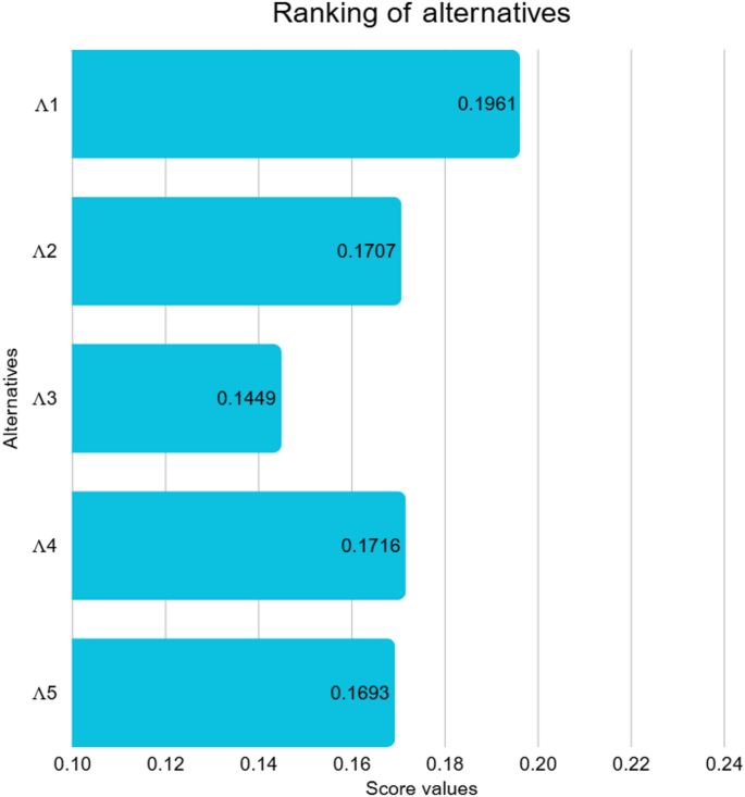
The proposed q-RLDF WASPAS approach provides a structured mechanism for evaluating, ranking, and recommending AI algorithms for PE by systematically capturing the interplay of multiple performance criteria in uncertain situations. Based on the final ranking obtained through our proposed methodology, the CNN-MA emerged as the most effective alternative, demonstrating superior capability in real-time motion tracking and posture analysis, which directly supports physical skill development and form correction. The RL-TO ranked second, reflecting its strong potential to personalize training regimens and adapt workout plans dynamically according to individual learner needs. The HAI-NLP secured the third position, showing promise in enhancing interaction and providing customized feedback through natural language interfaces. The remaining alternatives, WSDMA and the ES-EP, are positioned lower due to relatively limited adaptability and narrower application scopes within dynamic PE contexts. This ranking provides practical guidance for educators and administrators to prioritise AI solutions that best align with optimizing training effectiveness, learner engagement, and real-time performance monitoring in PE environments.