Mountain glaciers recouple to atmospheric warming over the twenty-first century

Weather station data

We obtain hourly on- and near-glacier air temperature (Ta) data for 169 individual glaciers over a range of years (1994–2023). Additional hourly meteorological data (for example, wind speed and relative humidity) are processed where available. Station data are either previously analysed in published articles and requested directly from the corresponding authors or are, at the time of writing, publicly available in online repositories (Supplementary Table 1 gives an overview of the datasets used)37. These data are obtained from AWS of varying complexity, or from small ‘T-Logger’ stations that record only Ta or Ta and relative humidity. For this study we refer to all on-glacier stations as an AWS for simplicity. We use data from AWS that are free-standing on the glacier surface, such that an ~2-m record of air temperature is maintained during the ablation season. Each AWS record is quality checked and erroneous data points are removed from the record. We retain all valid data points allowing data gaps and analyse the on-glacier AWS record for a given year when the following conditions are met:

The on-glacier AWS and its off-glacier counterpart AWS contain at least one complete month of hourly data (n ≥ 744).

The elevation difference between the on- and off-glacier AWSs is less than 1,000 m. This value was selected after manual inspection of the data to reduce uncertainty related to the local estimate of temperature given a 1 s.d. adjustment of the prescribed lapse rate (equation (1)). Data were also manually inspected to check that the off-glacier AWS is not subject to a regular occurrence of thermal inversions.

The off-glacier AWS is deemed to be outside the thermal influence of the glacier. We select off-glacier AWS that are situated ideally on a nearby moraine or, if in the proglacial area, are >700 m from the terminus of the glacier38. This distance was confirmed to be appropriate in recent analyses of off-glacier AWS data in proglacial areas14,21.

Derivation of ambient meteorological conditions

Ta data from the off-glacier AWS (TaOFF) are extrapolated to the elevation of the on-glacier AWS using a locally prescribed, hourly-variable lapse rate where available or the environmental lapse rate (ELR −0.0065 °C m−1) in the absence of the locally derived lapse rate values. We note that the ELR is broadly representative of the pressure, temperature, density and viscosity of Earth’s atmosphere over a wide range of altitudes and has often been used in the absence of locally available information about temperature changes with altitude. The calculation of the estimated ambient temperature (TaAmb) follows the form:

$${\rm{Ta}}_{\rm{Amb}}={\rm{Ta}}_{\rm{OFF}}+\varGamma \times ({z}_{\rm{Gla}}-{z}_{\rm{OFF}})$$

(1)

where Γ refers to the temperature lapse rate as above and zGla and zOFF are the respective elevations of the on- and off-glacier AWS.

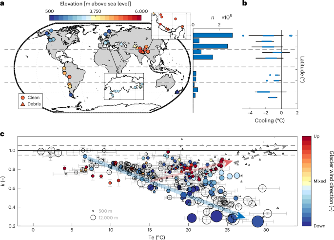
Mean atmospheric conditions are also represented by the equivalent temperature (Te; Fig. 1c), which represents the heat content near to the surface if all latent heat were converted to sensible heat20,39:

$${\rm{Te=Ta}_{Amb}}+\frac{\rm{Le}}{Q}{\rm{Cp}},$$

(2)

where Cp is the specific heat of air at constant pressure, Le is the latent heat of vaporization or sublimation and Q is the specific humidity derived from the available off-glacier AWS records. The value of Te helps to reconcile some of the expected differences in estimated and actual heat content at high elevation, humid regions (for example, the Tropical Andes and in southern High Mountain Asia) where latent heat release can modify the assumed lapse rate23,40 (see Results section: ‘Controls of temperature decoupling on mountain glaciers’ for interpretation of the role of humidity).

Temperature differences over glaciers

To provide a better estimate of the mean TaAmb at the equivalent on-glacier elevation, we calculate the mean bias of TaAmb and the observed Ta on the glacier (TaGla) under subzero temperatures (thus ignoring the conditions under which the relevant processes, that is katabatic winds, are occurring) and use that mean bias to correct all hours of TaAmb only (Supplementary Fig. 3b).

The calculation of the glacier decoupling factor k is based on the slope of the linear regression between TaAmb and TaGla (following refs. 10,14,21; Supplementary Fig. 3c):

$$k=\frac{{\rm{Ta}}_{\rm{Gla}}-{\beta}}{{\rm{Ta}}_{\rm{Amb}}}$$

(3)

where β is the intercept of the linear regression. A k value of 0.5 indicates that for every temperature increase of 1 °C outside the thermal influence of the glacier, a 0.5 °C increase would be observed at the near-surface over the glacier. Subsequently, the data points of k refer to the average value of decoupling during the unique summer/dry season considered per AWS. Mean cooling (MC) for the world’s glaciers (Figs. 3m and 4) is treated as the temporally and spatially averaged bias of TaAmb and TaAmb multiplied by k, such that a more negative value indicates a cooler near-surface Ta than the surrounding air (Supplementary Fig. 3a):

$${\rm{MC}}=\overline{\rm{Ta}}_{\rm{Amb}}\times k-\overline{\rm{Ta}}_{\rm{{Amb}}}$$

(4)

Glacier characteristics

To contextualize the spatial and temporal variability of glacier cooling and decoupling, topographic and climatological characteristics of each glacier are calculated for the point location of each AWS as well as for the glacier-wide average. A 30-m ASTER digital elevation model (DEM) was extracted from the NASA EarthData portal using the RGI18 v.6 outlines of each glacier. Outlines were manually updated in cases where large changes in length were observed over different periods of AWS observations on the glacier21. With this exception, DEMs and glacier outlines otherwise represent an average condition that corresponds to an earlier period (around year 2000 for RGI and 2011 for the DEM) than several of the AWS observations (Supplementary Table 1) but is deemed acceptable to describe the broad topographic characteristics.

Specifically, at each glacier, we calculate flowpath length (FPL (m); ref. 15), slope angle (SLP (∘), aspect (ASP (∘)), relative elevation expressed as the topographical position index (TPI (m)), as well as the elevation directly from the DEM itself (ELE (m above sea level)). Additional to the above, at each on-glacier AWS we consider the normalized FPL (nFPL (–)) which considers the flowpath distance adjusted by the maximum flowpath distance of the glacier, therefore expressing how far from the upper-most (0) or lower-most (1) portion of the ice body the AWS is sited. The up-glacier contributing area (uAREA (km2)) and mean up-glacier slope (uSLP (∘)) of each AWS is also extracted. The presence of debris cover is extracted from the database of ref. 19, although debris thickness is not considered.

Hydrometeorological characteristics

Hourly meteorological information is provided by ERA5-Land reanalysis at the nearest centroid pixel to the centroid coordinates of the glacier and air temperature is adjusted to the mean elevation of glacier DEM considering the pressure level temperatures of ERA5. Incoming shortwave (Swin (Wm−2)), longwave radiation (Lwin (Wm−2)), 10-m wind speed (FFERA (m s−1)) and direction (DIRERA (°)), air temperature (Ta (°C)) and dewpoint temperature (dTa (°C)) are used to assess prevailing conditions under which cooling is promoted or restricted. Specific humidity (Q (g kg−1)) is calculated from Ta, dTa and air pressure at the given elevation of the AWS. The mean isotherm elevation is calculated and used to explore the relative elevations (RELEL (m)) and relative flowpath lengths (RELFPL (m)) of the AWS points compared with this mean isotherm. Daily snow cover and albedo for each glacier are also obtained from MODIS MOD10A1 using the NASA AppEEARS toolbox, corresponding to the period of AWS observations and used to examine if the presence of snow cover has a notable impact on the degree of cooling.

A predictive model for temperature decoupling

A multiple linear regression model is built given k as the predictand and testing variations of the glacier topographic and meteorological predictors mentioned above. All predictors are either temporally invariant (for example, elevation and slope) or are averages of the meteorological conditions for the period of AWS data for a given year/glacier (for example, air temperature). Data from AWS points were iteratively subsampled using a random filter, allowing only a single AWS location on a given glacier for each iteration to avoid overfitting to glaciers with many observations in given years (Supplementary Table 1). For each iteration (n = 1,000) all predictors stated above were provided to a least absolute shrinkage and selection operator (lasso) regressor27 with a cross-validation scheme which determined the predictors to which k was most sensitive (Supplementary Fig. 18). The lasso regression tries to minimize the mean squared error, which is based on balancing the opposing factors of bias and variance (L1 penalty parameter weight λ) to build the most predictive model, shrinking the lasso parameter of less important predictors to zero. As λ increases, the bias increases and variance decreases, leading to a simpler model with fewer parameters.

The predictors that emerged from the scheme given that 1 s.d. of the mean λ were off-glacier air temperature, off-glacier specific humidity, synoptic wind speed from ERA5-Land (after bias correction; Supplementary Fig. 24), flowpath distance and elevation. These predictors were applied to a multilinear regression model that was iteratively cross-validated using three different strategies for the choice of subsampling, based on AWS distributions and the number of sample years for a given glacier. While the strength of individual predictors was impacted by the number of stations applied to sampling strategy, extensive testing found a stable score of predictability of k (Supplementary Section 4). The estimations of k using ERA5-Land data are compared for different glaciers in Supplementary Fig. 27. Following cross-validation, and for application to a global estimate (see the following section), we use all valid data points to build the ’full’ multilinear regression model. The final form of the ’full’ model, where xi are the regression coefficients, is:

$$k\approx {x}_{0}+{x}_{1}{\rm{Ta}}+{x}_{2}Q+{x}_{3}{\rm{FF}_{ERA}}+{x}_{4}{\rm{FPL}}+{x}_{5}{\rm{ELE}}+\epsilon$$

(5)

Nonlinear terms and machine learning approaches were tested with the available dataset, but resulted in small gains of predictive capability for the loss of wider applicability or interpretability, and were therefore not applied. The coefficients, errors and CIs of the model are provided in Supplementary Section 4.

Regionalization of temperature decoupling

To estimate mean temperature decoupling of the world’s mountain glaciers, we combine mean summer (June to September or December to March in the southern hemisphere) air temperature (TaERA), dewpoint temperature (dTaERA) and wind speed (FFERA) data from ERA5-Land for the 2000–2022 period with the glacier characteristic information from RGI v.618 and the equivalent debris cover classification from ref. 19. For each glacier centroid of the RGI, mean TaERA, dTaERA and FFERA were extracted and averaged over the 2000–2022 period. TaERA and dTaERA were downscaled to the elevation of the glacier in 50-m intervals between the minimum and maximum elevations of the RGI and using mean lapse rates from pressure levels of the equivalent ERA5 pixel (Supplementary Fig. 22).

The maximum length of each glacier was used to generate a range of flowpath distances starting at 0 m for the highest elevation point. The debris cover ratio was derived for each glacier and assigned to the equivalent elevation band, with the assumption that 90% of the total glacier debris coverage exists on the terminus of the glacier.

For each elevation band of each glacier the predictive model (equation (5)) was used to make an estimate of mean k over clean ice, maintaining an upper limit of 1 (fully coupled air temperature) and a lower limit of 0.2 (the minimum k value derived from the observations; Fig. 1c). Debris-covered elevation bands set to a value of 1 with a simple linear reduction of k based on the distance of the debris areas to up-glacier clean ice areas (Supplementary Fig. 14). Above-debris k values exceeding 1 (that is, additional warming due to the debris surface heating) were not considered. We use the 95% CI from the predictive model to provide an estimate of uncertainty for the resulting values of k.

Future climate scenarios

For each glacier we extracted a six-member ensemble of air temperature (TaCMIP), relative humidity (RHCMIP) and wind speed (FFCMIP) from middle of the road (SSP 2-4.5) and pessimistic (SSP 5-8.5) CMIP6 scenarios. The models used are: AWI-CM-1-1-MR, CMCC-CM2-SR5, CanESM5-CanOE, INM-CM5-0, KIOST-ESM and NESM3, all of which had projections of the above variables. We use the data from the pressure level most closely corresponding to the median elevation of each glacier for each model member. These data were bias-corrected against the ERA5-Land ‘observations’ using a mean additive approach during the period of 2000–2022 and subsequently downscaled to the elevations of the glaciers using the summer specific, mean linear lapse rates derived from the pressure levels of each model member and scenario (Supplementary Fig. 24). RHCMIP was converted to specific humidity (QCMIP) for input into the model. FFCMIP was considered static over the different elevation bands of the glacier and limited to the minimum observed value from FFERA if it was less. Glacier area and thickness changes from the ensemble mean of the SSP 2-4.5 and SSP 5-8.5 scenarios are taken from ref. 8 and used to adjust the surface height for the meteorological downscaling of TaCMIP and QCMIP and to limit the elevation bands over which k estimates are made in each year from 2000 to 2099. For future changes in glacier area, we consider the debris cover ratio and its distribution to be unchanged.