
Synthetic dataset
A synthetically generated PPG signal has been developed to provide precise control over the signal-to-noise ratio and the dynamics of heartbeats per minute. The signal was implemented approximating a single PPG pulse with two Gaussian functions51 and applying the circular motion principle to distribute PPG pulses over time. The overall dynamics can be described as:
$$\left\{\begin{array}{l}x\left(t\right)=cos\left(\omega \left(t-{t}_{0}\right)-\pi \right)\quad \\ y\left(t\right)=cos\left(\omega \left(t-{t}_{0}\right)-\pi \right)\quad \\ z\left(t\right)=\mathop{\sum }\limits_{i = 1}^{2}{a}_{i}{e}^{-\frac{{\left(\theta \left(t\right)-\theta i\left(t\right)\right)}^{2}}{2{b}_{i}^{2}}}\quad \end{array}\right.$$
(1)
where x(t) and y(t) describe a cyclic dynamics and ω = 2πν the angular velocity. z(t) is modeled as the sum of two Gaussians, representing the amplitude of the synthetic PPG signal, whit ai representing their peak values, 2bi their σ and \(\theta (t)=atan2\left(y(t),x(t)\right)\) as the angle in polar coordinates. The constants t0 and θi(t) define the initial conditions. Used parameters are reported in Table 1.
Table 1 Synthetic signal parameters
To determine the parameters of the synthetic PPG waveform, 10 events were randomly selected from a real PPG sample in the BIDMS dataset (trial bidmc01). A PPG pulse was defined as the data points between the midpoints of two consecutive valleys at the boundaries of a PPG event. The model was then fitted to each of the 10 selected events, and the final parameters were calculated as the averages of the fits: All experiments in this study involving synthetic PPG signals are based on the parameters reported above.
Noise
To simulate a continuous signal with added noise at varying SNR in decibels and to incorporate additional noise of specific colors, a systematic approach is followed. Based on the desired SNR in dB, the required noise power is determined using the relationship between signal power Psignal and noise power Pnoise, so that
$${P}_{noise}={P}_{signal}* 1{0}^{-SNR/10}$$
White noise, characterized by a flat power spectrum, is generated as a random Gaussian signal with zero mean and a variance Pnoise. This white noise is then added to the original signal, producing a noisy version of the signal for each specified SNR value. The procedure is repeated iteratively for multiple SNR levels, enabling the generation of noisy signals with varying degrees of noise intensity. To introduce additional colored noise, white noise is filtered to modify its spectral density. Finally, the colored noise is added to the previously generated noisy signals, producing a final signal that incorporates both white noise and colored noise.
Biomedical datasets
To test the networks implemented, we selected real-world datasets of PPG signals, choosing two complementary datasets to address different scenarios. The first dataset (BIDMC) provides clean measurements under controlled conditions, including a reliable ground truth heart rate. The second dataset (WristPPG) captures signals during dynamic activities with varying heartbeats. For this latter dataset, we developed a hardware-aware cleaning method leveraging accelerometer signals to mitigate motion artifacts (see “Motion artifact mitigation”).
To evaluate our model, we utilized a publicly available dataset from the IEEE Dataport, which contains multimodal recordings of EEG, PPG, blood pressure, and respiratory signals52. These recordings were collected from 53 subjects under various physiological conditions, including resting states and activities designed to induce changes in cardiovascular and respiratory dynamics, such as controlled breathing and postural changes. Each session lasted approximately 8 minutes, with all signals sampled at 125 Hz. Importantly, the signals provided in this dataset are relatively clean, as the controlled conditions minimize movement artifacts, reducing noise and simplifying signal processing. Additionally, the dataset provides a ground truth heart rate measurement sampled at 1 Hz, allowing for reliable validation of heart rate estimation methods.
To evaluate our model, we utilized a publicly available dataset containing left wrist PPG, chest ECG recordings, and motion data from accelerometers and gyroscopes53. These recordings were collected while participants engaged in physical activities using an indoor treadmill and exercise bike. The dataset captures various exercises, including walking, light jogging/running on a treadmill, and cycling at low and high resistance, with each activity lasting up to 10 minutes. The dataset includes recordings from eight participants, with most participants performing each activity for 4 to 6 minutes. All signals were sampled at a frequency of 256 Hz, and the ECG data underwent preprocessing with a 50 Hz notch filter to mitigate mains power interference. The interest of this dataset lies in the involvement of the subjects in dynamic activities, allowing us to observe significant variations in heart rate. On the other hand, these activities introduce substantial motion-related noise in the sensor data, posing a challenge for accurate signal analysis. It is important to note that the dataset lacks a ground truth reference for heart rate, further emphasizing the complexity of deriving reliable physiological metrics from these recordings.
Signal preprocessing
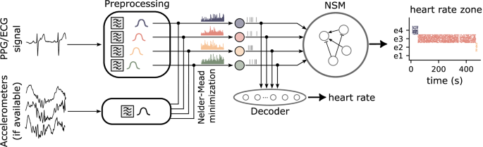
The signal preprocessing follows an energy-based approach for signal-to-spike conversion20,54. The procedure consists of two main stages: bandpass filtering and Leaky Integrate-and-Fire (LIF) neuron encoding55. Initially, each input channel is processed through a series of 4 bandpass filters to isolate frequency components corresponding to different heart rate bands, using fourth-order Butterworth filters. After filtering, the signal undergoes full-wave rectification, ensuring that the entire waveform is positive. The rectified signal is then amplified before being injected as a time-varying current into a Leaky Integrate-and-Fire (LIF) neuron, which integrates the current and encodes it as spiking activity. This encoding stage allows the continuous signal to be represented in discrete spikes, which can then be processed by subsequent layers of the neuromorphic system.
Such LIF neurons are governed by two key parameters: the neuron time constant τ and the neuronal spiking threshold Vthr. Throughout this study, we set these parameters to τ = 24ms and Vthr = 1. However, as shown in Fig. 6b, the system decoding performance remains stable across a range of parameter values for the preprocessing LIF. We intentionally chose parameter values that are far from the stability boundaries, even if they are not strictly optimal. Furthermore, working at a higher spiking threshold reduces the number of spikes, which is beneficial for power consumption.
Fig. 6: Impact of noise and LIF neuron parameters on signal reconstruction accuracy.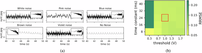
a Examples of synthetic signals with different types of noise for a Signal to Noise Ratio (SNR)=10. Synthetic signals with white noise (flat power spectrum), pink noise (power inversely proportional to frequency), blue noise (power directly proportional to frequency), brown noise (power inversely proportional to the square of the frequency), violet noise (power proportional to the square of the frequency), and the noise-free signal for comparison. Insets display the corresponding power spectral density for each noise type, highlighting the spectral characteristics. b Impact of Leaky Integrate-and-Fire (LIF) neuron parameters on decoder reconstruction accuracy. The heatmap illustrates the Relative Root Mean Square Error (RRMSE) of decoder reconstruction for different preprocessing parameters of LIF neurons. It represents the RRMSE between the reconstructed Heart Rate (HR) and the target HR for a synthetic signal. The decoder network processes input signals converted into spike trains by LIF neurons, with varying time constants and spiking thresholds.
For this study, we evaluated two different frequency band selections: one set of bands, consisting of 60-82 bpm (e1), 82-105 bpm (e2), 105-128 bpm (e3), and 128-150 bpm (e4), was chosen to cover a broad range of heart rate variations, from a relaxed state to tachycardia. In addition, to highlight subtle changes in heart rate and test the system’s ability to handle faster transitions, we also preprocessed the BIDMC dataset using narrower frequency bands: 60-80 bpm (e1), 80-88 bpm (e2), 88-96 bpm (e3), and 96-150 bpm (e4).
Motion artifact mitigation
Motion artifacts and noise significantly impact PPG signal quality, requiring robust preprocessing for reliable analysis56. Common methods include zero-phase Butterworth band-pass filtering (0.5-10 Hz) to remove noise, rolling standard deviation for artifact segmentation, and adaptive thresholding algorithms like a modified Pan-Tompkins for peak detection in challenging environments45,57.
In wearable devices, combining PPG with accelerometer data has become standard for addressing motion artifacts58,59. Accelerometers detect movement and correlate it with affected PPG segments, enabling precise artifact removal where traditional filters fail. Techniques like adaptive noise cancellation60, spectral comparison61, and machine learning models further enhance artifact removal by integrating PPG and accelerometer signals62.
To explore the dynamics of heart rate estimation in the presence of motion artifacts, we used the Wrist dataset, which includes simultaneous ECG and PPG recordings from eight subjects performing various physical activities. Given the motion-intensive nature of these exercises, the PPG signals were significantly affected by motion artifacts, which posed a challenge for accurate heart rate estimation. Although the dataset does not provide a direct ground truth for heart rate, we utilized the available ECG recordings as a surrogate reference.
To mitigate the impact of these motion artifacts, we utilized accelerometer data while addressing the constraints of low-power, always-on systems. In the absence of a true ground truth for heart rate, we leveraged the ECG recordings as a surrogate reference for heart rate estimation. Our methodology optimized a linear combination of the four bandpass-filtered PPG signals and the accelerometer data (one accelerometer per direction). The goal was to align the firing rates of the resulting LIF neuron outputs with those derived from the ECG. A comparison between each band’s ECG (i.e., target), PPG, and cleaned signals—optimized across all inputs, subject-specific, and exercise-specific—is shown in Figure 7, along with the spiking data output from each LIF neuron.
Fig. 7: Comparison of cleaned Photoplethysmography (PPG) signals across different processing stages.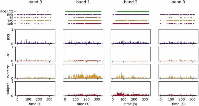
Each column represents a frequency band. The top row presents the corresponding spiking neuron outputs, illustrating the impact of motion artifact mitigation on neural encoding. Following rows show (from top to bottom) the raw Electrocardiography (ECG) (ground truth), raw PPG, and cleaned PPG signals optimized across all data, subject-specific, and exercise-specific settings.
The optimization process employed the Nelder-Mead algorithm48, a derivative-free method that is well-suited for optimizing complex, non-differentiable objective functions. The algorithm iteratively refines a set of simplex points to minimize the RRMSE between the firing rate curves derived from the LIF outputs and the reference ECG-derived firing rates. This approach avoids gradient-based methods, which are not ideal due to the overly smooth gradient landscape of the problem. Instead, we used random initialization followed by 20 iterations of optimization to converge on an optimal solution.
This method was applied to optimize the combination of signals either across all data samples or independently per subject or exercise type. Our results indicate that exercise-specific optimization yields performance comparable to subject-specific optimization, which enhances practical applicability. Although this traditional optimization approach is simpler compared to advanced methods, it yielded satisfactory results, balancing computational efficiency with the need for accurate removal of motion artifacts. Other approaches, such as deep learning models, require large amounts of data for training, while offline methods that analyze the full signal dynamics can be computationally expensive and less practical for real-time applications.
Computational primitives
E-I balanced networks provide a stable and adaptive computational basis for all architectures. They consist of tightly coupled excitatory (E) and inhibitory (I) neuronal populations that maintain a dynamic equilibrium between excitation and inhibition. This balance is critical for ensuring stability and preventing runaway excitation or excessive suppression within the network. In such networks, inhibitory neurons provide rapid feedback to counteract excitatory inputs, leading to precise control over the timing and magnitude of neuronal activity. This mechanism supports robust and stable computations while enabling the network to respond adaptively to input fluctuations, making E-I balanced networks fundamental in both biological and neuromorphic systems. Theoretical models63,64 suggest that cortical networks operate in a balanced regime, where excitatory and inhibitory inputs dynamically adjust to prevent runaway activity while maintaining responsiveness to stimuli. Mathematically, the total synaptic input to a neuron can be expressed as:
$${I}_{{\rm{total}}}={I}_{{\rm{exc}}}+{I}_{{\rm{inh}}}$$
where Iexc and Iinh represent the excitatory and inhibitory synaptic currents, respectively. In balanced networks, these contributions approximately cancel on average, leading to a net input that scales with external drive rather than diverging:
$$\langle {I}_{{\rm{exc}}}\rangle \approx \langle {I}_{{\rm{inh}}}\rangle$$
(2)
ensuring that fluctuations, rather than absolute magnitudes, dominate neuronal dynamics. The balance is often maintained through inhibitory feedback, which is modeled as:
$${I}_{{\rm{inh}}}=g{I}_{{\rm{exc}}}$$
(3)
where g is the inhibitory gain, typically greater than 1 in cortical networks. This ratio ensures that inhibitory neurons track excitatory activity and stabilize network dynamics.
Winner-Take-All is a computational primitive exploiting of competitive neural circuits in which a subset of neurons suppresses the activity of others, allowing only the strongest input to dominate the network’s response65,66. These networks are widely used in computational neuroscience and artificial neural systems for decision-making, feature selection, and clustering41,46,67,68. The dynamics of a WTA circuit can be described by the firing rate equations:
$$\tau \frac{d{r}_{i}}{dt}=-{r}_{i}+f\left({I}_{i}-\mathop{\sum }\limits_{j\ne i}{w}_{ij}{r}_{j}\right)$$
where ri represents the firing rate of neuron i, Ii is its external input, wij are the inhibitory connections between competing neurons, and f(⋅) is a nonlinear activation function. The competition arises from strong lateral inhibition, typically modeled as:
$${w}_{ij}=\gamma {{\Theta }}({r}_{j}-{r}_{i})$$
where γ controls the inhibition strength and Θ(⋅) is the Heaviside step function, ensuring that only the most active neuron suppresses others. In an idealized case, the network converges to a state where only the neuron with the largest input remains active, while all others are silenced:
$${r}_{k} \,>\, 0,\quad {r}_{j\ne k}=0,\quad \,{\text{where}}\,\quad k={\arg} \mathop{\max }\limits_{i}{I}_{i}.$$
This competitive mechanism enables efficient selection of the most salient input while filtering out weaker signals. Variants of WTA networks incorporate stochasticity, adaptive thresholds, or continuous soft competition to improve robustness and flexibility.
Neural State Machines are a class of neural architectures that encode discrete internal states and transition dynamics, enabling robust sequential decision-making, memory, and hierarchical processing6,47,69. Unlike traditional feed-forward networks, NSMs maintain internal state representations that evolve over time based on both external inputs and recurrent feedback. The core dynamics of an NSM can be described by a state update equation:
$$s(t+1)=f\left({W}_{s}s(t)+{W}_{x}x(t)+b\right)$$
(4)
where s(t) represents the hidden state at time t, x(t) is the external input, Ws and Wx are the recurrent and input weight matrices, respectively, b is a bias term, and f(⋅) is a nonlinear activation function. State transitions in NSMs often follow a probabilistic or soft-competitive mechanism, where the likelihood of transitioning to a new state depends on an energy function:
$$P(s_{t+1} | s_t, x_t) = \frac{\exp(-E(s_{t+1}, s_t, x_t))}{{\sum}_{s^{\prime}} \exp(-E(s^{\prime}, s_t, x_t))}$$
(5)
where E(st+1, st, xt) represents an energy function defining the cost of transitioning between states. This formulation allows NSMs to incorporate probabilistic state transitions, making them robust to noise and uncertainty. To enforce stability and prevent excessive state transitions, an inhibitory competition mechanism is also introduced:
$${I}_{{\rm{inh}},i}=g\mathop{\sum }\limits_{j\ne i}{w}_{ij}{s}_{j}$$
(6)
where g is the inhibitory gain, wij represents inhibitory coupling between states, and sj is the activation of competing states. This ensures that only a subset of states remains active at any given time, preventing unstable oscillations. In addition to their fundamental state-machine-like behavior, NSMs can process asynchronous events directly, without the need for clocked transitions. This capability allows NSMs to take advantage of sparse and slowly changing signals, reducing computational overhead and improving energy efficiency while also taking advantage from the distributed and parallel nature of spiking neural networks, making them more resilient to faults and noise. By combining recurrent dynamics, competitive inhibition, and probabilistic transitions, NSMs provide a powerful framework for modeling adaptive and memory-dependent behaviors in both biological and artificial systems70.
The Neural State Machine architecture
This section introduces the architectures underlying the NSMs, highlighting their unique features and operational principles. Each model builds upon fundamental neuromorphic computing principles to address distinct requirements in encoding and transitioning between heart rate bands (parameters in Table 2).
Table 2 Network parameters for the three architectures: Winner-Take-All (WTA), Nearest Neighbors Neural State Machine (nnNSM), and Monotonic Neural State Machine (monoNSM)
This WTA framework is designed to encode distinct heart rate bands using a competitive dynamic among its excitatory populations (e1,e2,e3,e4), as shown in Fig. 3a. Each excitatory population is tasked with representing a specific HR band, and the activation of one population suppresses the activity of others, ensuring only one HR band is active at any given time. The network employs a global inhibitory population (inh) to enforce this competition, where inhibitory signals uniformly suppress all excitatory populations, preventing simultaneous activation. This architecture is suitable for hard transitions between states and is highly effective in competitive environments. However, it lacks the mechanisms necessary for smooth transitions between adjacent states, which can be a limitation when dynamic and gradual changes in HR bands are required.
The nnNSM, depicted in Fig. 4a, is based on the WTA architecture augmented with disinhibition mechanisms to enable smooth transitions between adjacent HR bands. The nnNSM architecture consists of excitatory and disinhibition populations. As in the WTA architecture, the excitatory populations are responsible for encoding specific HR bands, with each population dedicated to a distinct frequency range and a global inhibitory population enforces competitive dynamics across the network. Differently to the WTA network, to facilitate smooth transitions and suppress competing activity, each excitatory population is also paired with a disinhibition population (disinh0, disinh1, disinh2, disinh3). The disinhibition populations are composed of an excitatory-inhibitory (E-I) balanced network. This reciprocal inhibition mechanism ensures that the network transitions seamlessly between adjacent HR bands while suppressing activity in non-adjacent bands. Together, the local disinhibition and global inhibition mechanisms enable the network to maintain a balance between sensitivity to input signals and stability in its dynamics. This mechanism avoids abrupt switching and maintains smooth, context-sensitive HR band selection. To further illustrate this, Fig. 8a presents a raster plot of the disinhibition E-I populations and the state network activity in response to biomedical data, highlighting the role of disinhibition in regulating smooth HR band transitions.
Fig. 8: Disinhibition populations activity in Neural State Machines.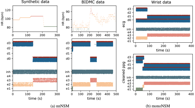
a Top: Heart Rate (HR) ground truth for synthetic (left) and real BIDMC (right) dataset. Bottom: Rasterplot of the monotonic Neural State Machine network showcasing the disinhibitory populations activity (d0, d1, d2, d3) for both excitatory (blue) and inhibitory (red) neurons together with the excitatory state-populatons (e1,e2,e3,e4) and global inhibition (inh). Bottom: activity when presented with cleaned Photoplethysmography (PPG) input. b Rasterplot of the monotonic Neural State Machine network showcasing the disinhibitory populations activity (d0, d1, d2, d3) for both excitatory (blue) and inhibitory (red) neurons together with the excitatory state-populatons (e1,e2,e3,e4) and global inhibition (inh). Top: activity when presented with Electrocardiography (ECG) input. Bottom: activity when presented with cleaned PPG input.
The monoNSM, illustrated in Fig. 5, builds upon the WTA architecture, incorporating a hierarchical structure and tailored input routing to support monotonic state transitions. In this setup, the excitatory populations are interconnected through asymmetric lateral inhibitory pathways, enforcing unidirectional transitions between states, which aligns with the monotonic progression. This organization promotes stability and efficient transitions, crucial for dynamic HR tracking under scenarios requiring strict band ordering. The monotonic NSM leverages these mechanisms to offer a robust yet adaptable framework for applications demanding structured state changes while maintaining low computational complexity. Similarly, Fig. 8b displays a raster plot of the state network activity in response to wrist dataset, showcasing how the asymmetric inhibitory pathways enforce ordered state transitions while preserving stability.
The DYNAP-SE neuromorphic hardware
The neuromorphic processor used in this study is the DYNAP-SE chip, a multi-core asynchronous mixed-signal neuromorphic processor designed to emulate the biophysical behavior of spiking neurons in real-time15. Each of its four cores contains 256 Adaptive Exponential Integrate-and-Fire (AdExp-IF) silicon neurons, with each neuron equipped with two excitatory and two inhibitory analog synapses. Synapses in the DYNAP-SE can be configured as slow/fast and inhibitory/excitatory, offering flexible functionality. Additionally, neurons within each core share common bias settings, resulting in shared time constant values. To facilitate communication, each neuron integrates a Content Addressable Memory (CAM) block with 64 addresses, representing its pre-synaptic connections. The chip uses the Address-Event Representation (AER) protocol for asynchronous communication71. In this system, each neuron is assigned a unique digital address transmitted asynchronously upon generating an event. The DYNAP-SE’s fully asynchronous inter-core and inter-chip routing architecture supports flexible and precise connectivity with microsecond-level timing, even under heavy system loads.
Power consumption
The power consumption of the DYNAP-SE cannot be directly measured during online operation, however, we can indirectly assess it as the sum of the required power for spike generation and communication72,73, as listed in Table 315:
$$P=\mathop{\sum }\limits_{n=1}^{N}{r}_{n}\left({E}_{{\rm{spike}}}\,+\,{E}_{{\rm{enc}}}\,+\,{N}_{{\rm{cores}}}\left({E}_{{\rm{br}}}+{E}_{{\rm{rt}}}\right)\,+\,{N}_{{\rm{cam}}\_{\rm{match}}}\,{E}_{{\rm{pulse}}}\right),$$
(7)
where: Espike, Eenc, Ebr, Ert, Epulse are the energy costs estimated via circuit simulations, for generating a spike, encoding and appending destinations, broadcasting within the same core, routing to a different core, and extending the output pulse, respectively. N denotes the total number of neurons int he network, rn is the firing rate of neuron n, \({N}_{{\rm{cores}}}\) refers to the number of cores each neuron’s spikes are sent to Ncam_match is the total number of postsynaptic neurons that receive the input spikes.
Table 3 Estimated energy consumption of the DYNAP-SE circuit operations15Performance evaluation metrics
To assess network performance, we employ the RRMSE, a normalized metric that quantifies the deviation between predicted and actual heart rate values. RRMSE is computed as the Root Mean Square-Error (RMSE) divided by the mean of the observed values, providing a scale-independent measure of accuracy. An RRMSE of 0 indicates perfect agreement between predictions and observations. It is defined as follows:
$${\text{RRMSE}}\,=\frac{\root\of{\frac{1}{N}\mathop{\sum }\nolimits_{i = 1}^{N}{({y}_{i}-{\hat{y}}_{i})}^{2}}}{\bar{y}}$$
(8)
is the mean of the observed values. Specifically, y represents the predicted heart rate values, \(\hat{y}\) denotes the actual heart rate values (i.r. ground truth), N is the total number of observations, and \(\bar{y}\) is the mean of the observed values.
Statistics
All on-chip results were repeated three times on three separate days to ensure robustness. Noise analysis was performed using 10 different seed initializations across the entire synthetic dataset. All reported means were calculated by averaging the mean values across dataset trials for each repeated measurement, while the standard deviations were computed as the average standard deviation across the repeated measurements. To empirically validate the robustness of our approach, we conducted repeated measurements across multiple independent chip initializations on different days. Since each power-on leads to a new parameter configuration, this procedure allowed us to systematically assess the system’s ability to cope with noise and variability in the hardware.
Network parameters
To ensure reproducibility and facilitate implementation, we provide a comprehensive overview of the key parameters used in our network models. The table below details neuron counts and connection probabilities for three architectures: WTA, nnNSM, and monoNSM. These parameters define population sizes, input connections, and disinhibition mechanisms, serving as a reference for model replication.