
Study area and disease data
Our analyses paired site-level estimates of tick density, tick-borne pathogen prevalence, and small mammal communities from 24 climatically and ecologically variable NEON sites (S1 Fig; S1 Table) located in the eastern United States (i.e., east of the 100th meridian) with county-level human case counts of TBDs collected by the CDC (from 2014 to 2018 for anaplasmosis and ehrlichiosis, 2014–2017 for babesiosis, 2014–2022 for Lyme disease). Biodiversity data from NEON were filtered to match the years for which corresponding disease data were available. The study area included 22 counties in 15 states across the eastern U.S. within the ranges of I. scapularis and A. americanum (S1 Table). Not all counties were sampled every year. For details on the temporal coverage per county, see Table S1. The total population of these counties is approximately 2,910,976 (2022), and reported cases comprised 2,171 of Lyme disease, 221 of anaplasmosis, 73 of ehrlichiosis, and 53 of babesiosis. Mean reported cases per 100,000 people were 0.0274 for Lyme disease, 0.0045 for anaplasmosis, 0.0012 for ehrlichiosis, and 0.0005 for babesiosis. Given that the CDC only reports human cases that were treated by a doctor and that infected individuals are more likely to see a doctor if they exhibit symptoms, we will regard the response variable in our models as disease prevalence rather than simply infection prevalence. TBD case definitions by the CDC include both confirmed and probable cases, to address under-reporting. Sampling protocols for tick, tick-borne pathogens, and small mammals are described in NEON sampling documents and are summarized in the Supplemental Methods.
Predictors
We downloaded the 2023 NEON data release for (i) tick drag surveys (DP1.10093.001), (ii) tick pathogen status (DP1.10092.001), and (iii) small‑mammal box trapping (DP1.10072.001) using the neonUtilities R package34 on 7 March 2024. We restricted all datasets to counties within the contemporary U.S. ranges of Ixodes scapularis (blacklegged tick) and Amblyomma americanum (lone star tick) in the eastern United States35,36 (approx. east of the 100th Meridian; see Supplementary Figure S1 and Supplementary Table S1 a map and list of sites). A brief overview of the NEON data processing framework can be found below, with details on the implementation included in the Supplementary Methods.
For the tick drag survey data, we retained only samples without compromise flags (e.g., acceptable sample condition). When some individual ticks were identified to the genus level but co‑occurred with only a single focal species in that sample, we assigned them to that species. For each site‑plot‑year, we calculated tick density as individuals per m² based on the highest observed count, standardized by the mean sampled area for each plot and year (see Supplementary Methods for details). We used the small‑mammal dataset to estimate (a) species richness (coverage‑based) and (b) relative abundance by county and year. We excluded samples with evidence that traps were not properly set or were disturbed, and computed total sampling effort as trap nights aggregated by county and year (see Supplementary Methods). Given that sampling effort varies across NEON sites, we used coverage‑based estimates of species richness with the iNEXT R package37,38 (see Supplementary Methods).
We calculated relative abundance for (i) all small mammals combined, (ii) white-footed mouse (Peromyscus leucopus), and (iii) eastern chipmunk (Tamias striatus), the last two being the most important reservoirs for Borrelia burgdorferi and Anaplasma phagocytophilum. To avoid inflating abundance with repeat captures of the same individual, we counted only first captures when estimating the relative number of individuals per species (see Supplementary Methods). Although capture-recapture models would be the ideal method for comparing across sites, many site‑year combinations have few or no recaptures, which makes capture–recapture estimators unstable. However, we believe that our minimum abundance index is a good alternative given our objective of providing a standardized proxy for relative abundance across sites. Finally, at 13 eastern NEON sites, subsets of nymphal ticks were screened annually (2014–2021) for zoonotic pathogens using 16 S rRNA amplicon sequencing. We retained only samples that confirmed hard-tick DNA, and estimated pathogen prevalence as the sample prevalence of tested nymphs for Borrelia burgdorferi (see Supplementary Methods). Borrelia burgdorferi prevalence entered the Lyme disease structural equation models (see Statistical Analyses). For tested pathogens and yearly sample sizes, see Supplementary Table S3.
As white-tailed deer are the assumed main reservoir host for E. chaffeensis16, and the primary reproductive stage host for I. scapularis39, we also included the most recent white-tailed deer density estimates for the United States (2001–2005) from the Quality Deer Management Association hosted by the U.S. Forest Service40. In this dataset, deer density is separated into four distinct ordinal categories: <15 deer per square mile, 15–30 deer per square mile, 30–40 deer per square mile, and > 45 deer per square mile40. In all cases, the more parsimonious model (lower AICc) treated deer density as a continuous rather than an ordinal variable.
Testing of pathogen prevalence in ticks occurred at 13 sites in the eastern U.S. (Table S2), starting in 201441. At the time of data analysis, tick pathogen prevalence was only available for 2014–2021. At a given site, a subset of sampled nymphal ticks was tested annually for the presence of zoonotic pathogens (Table S2). Pathogen status in nymphal ticks was tested using next-generation sequencing and 16 S rRNA primers. As quality control, we excluded all pathogen status results that did not also test positive for hard-tick DNA. Pathogen prevalence at a site was estimated as the proportion of nymphal ticks that tested positive for a given pathogen. Borrelia burgdorferi data were used to incorporate the prevalence of infected ticks into Lyme disease piecewise structural equation models (see below).
As climatic predictors for our analyses, we used NEON site coordinates to download temperature and precipitation using the “download_daymet_batch” function of the “daymetr” R package42. We then used these data to calculate the mean annual temperature and annual precipitation for each NEON site and year.
Statistical analyses
All statistical analyses were conducted in R version 4.3.243 To achieve our first goal of determining the combination of host and vector community variables that best explain human TBD prevalence, we used generalized linear mixed effects models (GLMMs) with a binomial error distribution to investigate patterns in human TBD prevalence associated with tick densities, main reservoir host abundance, and small mammal richness, with mean each NEON site’s mean annual temperature and annual precipitation as covariates, and county as a random intercept in all models. We included the county as a random intercept to account for repeated sampling over multiple years. As a measure of reservoir host abundance, we used the relative abundance (for small mammals) or density category (for the white-tailed deer) of each disease’s primary competent reservoir hosts: white-footed mice for Lyme44, white-footed mice and eastern chipmunk for anaplasmosis17, all small mammals for babesiosis15, and white-tailed deer for ehrlichiosis16. We included small mammal richness as a predictor of ehrlichiosis strictly as a control for small-mammal diversity effects, as small mammals are not known to be as competent reservoirs as deer. Because adult I. scapularis ticks feed on deer, we also added deer density for diseases vectored by this tick. For the full Lyme disease and anaplasmosis models, we used “glmer” in the “lme4” package45.
For the Babesiosis and Ehrlichiosis models, we initially fit binomial GLMMs using “glmer”, but encountered singular fit warnings, indicating that at least one variance component was estimated as zero. Follow-up inspection revealed that the variance associated with the random intercept for County was collapsing toward zero. This behavior might reflect identifiability and overparameterization challenges, likely due to the sparsity of data for these two diseases: Babesiosis cases averaged 0.9 per county-year (maximum = 18), and Ehrlichiosis cases averaged 0.84 (maximum = 23). Because the same counties were sampled across multiple years, we retained the random intercept to account for temporal dependence. To address the singular fit warnings, we used a weakly regularized Bayesian approach implemented in “bglmer” (package blme46, specifying a weakly informative gamma prior (shape = 2.5, rate = 0) on the random-effect precision. This prior helps stabilize estimation of variance components in cases where the data provide limited information, while still allowing the data to inform the extent of random-effect variation. Given that the variance component for County is only weakly identified for babesiosis and ehrlichiosis, results involving this random effect should be interpreted with caution.
To improve the interpretability of unstandardized estimates with small per-unit effects, annual precipitation was expressed in 100-mm units, small-mammal relative abundance in 100-trap-night units, and tick density in 100-m² units. Conditional and marginal R2 were obtained using the method from Nakagawa et al.47 and implemented in the “performance” R package48.
Model assumptions
We used the DHARMa R package49 to look for evidence of assumption violations in our models, including multicollinearity, overdispersion, zero inflation, non-uniform variance, or spatial autocorrelation (see Supplementary Code for implementation and outputs). Collinearity was evaluated both before and after model fitting: prior to fitting, we examined pairwise correlations among predictors, and after fitting, we calculated variance inflation factors (VIFs) (see Supplementary Code for implementation).
Direct and indirect effects
To address our second objective of direct and indirect effects of tick density and reservoir host metrics on human disease prevalence, we used the piecewise Structural Equation Modeling (pSEM) framework. Because of sample size limitations for anaplasmosis, babesiosis, and ehrlichiosis, we limited this analysis to Lyme disease. All predictors were standardized before the analysis, and all four models included county as a random intercept. The structural equation model was fitted using the “psem” function of the “piecewiseSEM” package using the error distribution that was appropriate for each dependent variable50.
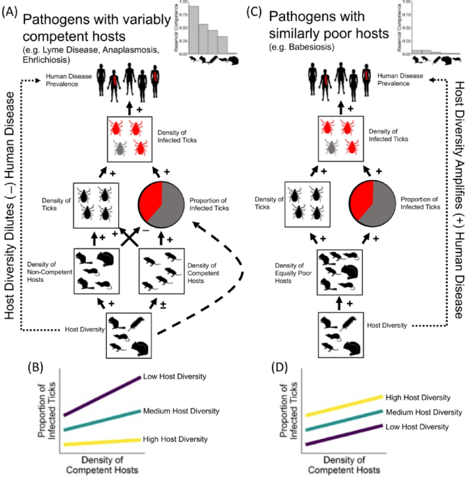
We specified our SEM a priori, grounded in well-established ecological theory on Borrelia transmission dynamics and supported by national‐scale analyses (Fig. 1; refs13,18,22,51. Four linked sub-models comprised our full causal structure (schematic in Fig. 5; refs13,18,22,51:
1.
Lyme prevalence in humans ~ density of infected ticks + B. burgdorferi prevalence in ticks + mean annual temperature + annual precipitation. This model assumes that the density of infected ticks directly influences reported human cases52 and that higher prevalence increases the likelihood that any tick bite is infectious53, independent of tick density. Additionally, we included climate as it might influence human outdoor behavior54.
2.
Density of infected ticks ~ density of ticks + B. burgdorferi prevalence in ticks. The density of infected ticks depends on the density of ticks and the B. burgdorferi prevalence in the population.
3.
Density of ticks ~ deer density + white-footed mouse relative abundance + relative abundance of non-competent hosts + mean annual temperature + annual precipitation. Deer density was included because deer are the primary hosts for adult ticks23,24,39, while white-footed mice and non-competent hosts can influence the number of nymphs present in the vegetation15. Temperature and precipitation were included due to their direct effects on tick survival, which ultimately determine tick density55.
4.
B. burgdorferi prevalence in ticks ~ white-footed mouse relative abundance * relative abundance of non-competent hosts + mean annual temperature + annual precipitation. The interaction term was included because the dilution effect depends on the relative composition of competent versus non-competent hosts rather than their absolute abundances51,56. Temperature was included, given its documented influence on Borrelia transmission efficiency57.
D-separation tests indicated a residual association between the density of infected nymphs and B. burgdorferi prevalence in ticks that was not captured by our directed paths (t₄₈ = −3.57, p = 0.0004). Because we lacked a causal mechanism for direct density dependence of tick prevalence, we incorporated this as a correlated error term, accounting for unmeasured shared influences without implying directionality.
Disability-adjusted life years (DALYs)
For models with significant effects of small mammal richness on human disease prevalence, we calculated the differences in case prevalence from 2022 (the year with the most recent complete data) by subtracting the median county-level prevalence from the counties in our dataset for a given disease in 2022 from the model-predicted prevalence. We then multiplied this relative change in prevalence by the average population within counties in our dataset to get the average change in disease incidence across counties. Change in Lyme disease incidence was then converted to change in annual disability-adjusted life years (DALYs) to provide an estimate of average county disease burden from changing disease incidence. Average case DALYs for Lyme disease have been estimated for patients with different Lyme disease outcomes: erythema migrans (0.005 DALYs), disseminated Lyme disease (0.113 DALYs), and Lyme-related persisting symptoms (1.661 DALYs)58. Relative prevalence of these outcomes per Lyme disease diagnosis is 82.8% for erythema migrans, 8.6% for disseminated LD, and 8.6% for persisting Lyme disease symptoms6. Thus, the estimated DALYs per Lyme disease case is 0.156.