
There are challenges to validating these data, as there is no “ground truth” dataset of state legislative bills coded under the Gray and Lowery codebook. This presents two issues: first, translating between disparate codebooks introduces measurement error, as bills could be “correctly” assigned according to each codebook but not translate to each other. For example, the Gray and Lowery codebook has a category for electric utilities (“Utilities”) that is separate from the PPDP’s “Energy” topic, so any bill assigned to utilities could be labeled as incorrect. Second, the complexity of assigning bills to a single policy area is a demanding task on its own. Many state politics researchers have deemed the classification task complex enough to necessitate that a domain expert inspect documents by-hand. For example, Reingold et al. (2021)25 first applies a dictionary method to identify legislation concerning abortion by searching for the “abortion” keyword, and then their second stage of analysis requires hand-coding bills to measure their abortion “sentiment.” The Congressional Bills Project1 and the codebook to which it adheres do away with keywords entirely, instead training hand-coders for several weeks to identify the leading policy area of the bill. This approach has its own issues, first it is not 100 percent reliable. Hillard et al. (2008, p. 40)15 report that coders are trained until they code congressional bills by 21 major topic codes at 90 percent reliability, and the 200+ minor topic codes at 80 percent reliability. Second, using hand-coders comes at the expense of transparency; unless the project clearly annotates the “why” for each hand-coder classification decision, it is difficult to diagnose hand-coder versus downstream researcher disagreements.
To address these concerns we take the following steps to demonstrate the validity of these estimates. First, we compare the machine learning model’s estimates to the legacy dictionary method. This shows how the machine learning model offers similar levels of precision, which provides confidence that the model is finding the policy content it is claiming to, but far better recall, or the degree the model is finding all possible bills in each policy area. Second, we compare the model to estimates generated by hand-coders16 to show that the model is reliable.
These exercises demonstrate the external validity of these estimates such that machine learning estimates track the hand-coded estimates of the Pennsylvania legislature closely over time. In particular, the machine learning greatly outperforms the legacy dictionary method in its recall of potential bill codings.
Model Evaluation Against Legacy Dictionary Method
We first evaluate the machine learning estimates against the legacy dictionary method. This is not a traditional validation, as the dictionary method is less of a “ground truth” than an alternative approach. But by showing which policy areas these two models agree and disagree on, we can better understand how the machine learning model operates. In Table 3, a “false positive” denotes an instance where the model predicts the presence of a given topic despite the absence of all its keywords. A “false negative” denotes an instance where the model predicts the absence of a given topic despite the presence of one of its keywords. “True positives” and “true negatives” are cases where the model and dictionary method agree to assign or not assign the topic to the bill, respectively.
Table 3 Model performance evaluated against the legacy dictionary method.
For almost all topics, false positives outnumber true positives, owing to the fact that the legacy dictionary method generates codes for a much smaller share of bills. A higher topic Precision denotes a larger share of true positives compared against all positives; as Precision increases, the model finds fewer instances where it predicts the presence of a topic despite the absence of keywords, meaning the keywords are more “necessary” for identifying the topic. For example, the most precisely-defined topic, by far, is “Tax Policy”, with Precision = 74%. It may be hard-pressed to think of a bill pertaining to “Tax Policy” which lacks all mentions of “tax,” “taxation,” “taxable,” and so-on (or at least, it may be harder to find such instances than it would be to find counterparts in other topics), but there are “Tax Policy” bills that include mentions of a “levy,” “Department of Revenue,” “economic development,” or “bonds.”
The lowest precision topics are “International Affairs and Foreign Aid” (5%), “Law” (6%), and “Civil Rights” (13%), meaning the model frequently predicts the topics’ presence without keywords being present. To shed light on whether these overrides of the dictionary method’s keyword rules are valuable, “International Affairs and Foreign Aid” (abbreviated in the table as “Intl. Affairs”) often include “exchange programs” (for students), explicitly mention other countries, or include other nouns plausibly associated with international affairs. For example, the dictionary defined in Table 1 includes the keywords “diplomat” and “embassy,” but not “ambassador,” and yet, “ambassador” takes on a similar semantic meaning with respect to the machine learning model’s classification task. Using the keywords associated with the “Civil Rights” topic as its conceptual “seeds,” the model has grown the topic to include a large number of resolutions, especially those which “celebrate the life” of an individual, mention “slave trade,” “equal opportunity,” or “human rights.” The multi-label nature of the data proves especially useful in flagging e.g. a bill which mentions “Female Veteran’s Day” as pertaining to both “Civil Rights” and “Military,” and a bill mentioning the “Equal Opportunity Scholarship Act” as pertaining to both “Civil Rights” and “Education.” False positives for “Law” often discuss “liability,” “unenforceable,” “covenant,” “contract,” “Juvenile Justice,” and “allegations.”
To provide a high-level perspective the internal consistency of the model, Fig. 6 presents a heatmap of topic co-occurrences for bills for which no keywords are present. Using non-keyword-coded bills illustrates that how the model performs without the strongest clues regarding policy areas. For each of the figures, a cell value denotes the percentage of bills coded as Topic = Row which were jointly coded as Topic = Column. For example, the “Civil Rights” topic most frequently co-occurs with “Religion,” “Law,” and “Labor and Employment,” even when of whether the bills contain zero keywords. The other top co-occurrences are “Environment” and “Public Lands and Water Management” and “Sports” (often with references to fishing and hunting), “Health” and “Insurance,” “Foreign Trade” and “Manufacturing,” “Construction” and “Utilities,” as well as “Natural Resource” and”Environment.” The “Utilities” topic most often co-occurs with “Communication” (e.g. telecomms) and “Local Government.”
Fig. 6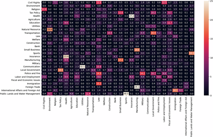
Correlation between topics based on model predictions, no keywords. Notes: Cells denote the frequency with which bills predicted as pertaining to Topic = Row are also coded as Topic = Column by the model, observing only bills for which there are no keywords present from either Topic = Row or Topic = Column. For example, 12.8% of bills which were predicted as pertaining to “Religion” (while lacking any “Religion” keywords) were also coded as pertaining to “Civil Rights” (while lacking any “Civil Rights” keywords).
Internal Validation
To demonstrate the face validity of the data, we drill down into the estimates with an issue that has emerged in the years since the original dictionary codebooks were published: fracking. Fracking developed as a political issue in the US following the development of “hydraulic fracturing” or “hydrofracking” technology in the mid-2000s allowed for energy companies to take advantage of shale underneath many, but not all, American states to produce natural gas and oil. While this was a revolutionary technique for energy extraction, it also had concerning environmental consequences, as the chemicals used for fracking, and its byproducts, could be toxic for groundwater and other environmental factors.
To test for fracking being accounted for by our model, we look to see if bills containing the many synonyms for this new technology are coded in the categories we would expect. We identify fracking bills using the following (case-insensitive) search terms in bill titles and descriptions: fracking, hydro fracturing, hydro-fracturing, hydrofracturing, hydro fracking, hydro-fracking, hydrofracking, hydraulic fracturing, hydraulic-fracturing, shale gas, shale oil, horizontal drill, horizontal gas, horizontal stimulation, horizontal well, fracturing fluid, fracturing wastewater, fracturing water, and fracturing chemical. At least one of these search terms appeared in 736 bills from 2009-2020. We find that the model assigns them in logical categories. Figure 7 illustrates that the fracking-related search terms are mostly concentrated to the “Energy or Natural Resource” and “Environment” topics, there is also some prevalence in “Public Lands and Water Management”. We take this exercise as further evidence’s of the model’s internal reliability.
Fig. 7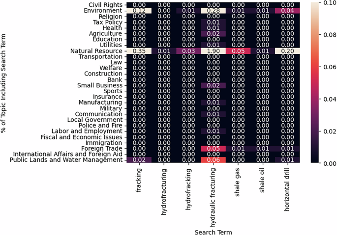
Topic hit rate for example search terms related to “Fracking.” Notes: A cell denotes the percentage of bills predicted to be assigned to topic = row that include the (case-insensitive) search term associated with its column.
A human coder also evaluated a sample of 1,000 randomly selected bills drawn from a separate database (OpenStates) to 1) evaluate the completeness of the sample drawn from Legiscan, 2) allow for the comparison of a multi-class system, 3) provide feedback on the uncertainty of the process. This exercise produced a number of results. First, it showed that Legiscan contained 100 percent of the bills in the OpenStates archives, which reaffirms our decision to take the Legiscan data at face value. Second, the human coder revealed the difficulty of these coding decisions. The human coder was provided the same bill title from legiscan that the model was fed, and was asked if this was sufficient to assign a bill or if it was necessary to look up the full text of the bill via a link to its pdf. On 25.4% of bills, they required the full text. This was not data that the model had access to. Third, they were instructed to place the bill into a single category, if feasible, or if the bill was too complex, to assign a second category. They found that 44% of bills required a second category.
We evaluate the accuracy of the model in two ways designed to evaluate multi-label prediction models26. First, we estimate the model’s “Ranking Loss”, which calculates the average number of incorrectly labeled pairs. For example, the hand-coder assigned Alabama’s “Property Insurance and Energy Reduction Act” (SB 220 from 2015, titled: “Energy efficiency projects, financing by local governments authorized, non ad valorem tax assessments, liens, bonds authorized, Property Insurance and Energy Reduction Act of Alabama”) as “Natural Resources” and “Local Government”, but the model’s first two estimates were “Utilities” (τ = 0.98) and “Tax Policies” (τ = 0.42). Since “Local Government” (τ = 0.16) was the third highest estimate, the ranking loss for this bill was 2. A perfect classifier would be zero, and chance would be 0.5. The average ranking loss for this sample of bills was 0.043, an impressive score.
Another way to conceive of multi-label classifier is through Top-K agreement, which indicates the share of times the hand-coder assigns the bill to a variable (K) number of classes. The previous example would be a bill that does not find agreement at K=1 or K=2, but does find agreement at K=3. Table 4 shows how if only the top option is included, there is agreement between the human coder and model estimates on 57 percent of bills. If the first three model estimates are considered there is agreement on 80 percent of bills. This is similar to the Policy Agenda Project’s considers to be suitable for human coder performance on minor topic codes.
Table 4 Top-K agreement of model estimates and human coded sample (n=1,000).
The accuracy and precision of the model can also be calibrated using different tau cutoff rates. Table 5 shows the range, and the default level (τ = 0.5). A higher tau would only provide more confident estimates, at the expense of total coverage. The lower F1 scores can be considered an artifact of the multi-label to multi-label comparison.
Table 5 Evaluation of machine learning estimates (at different levels of τ against human coded sample (n=1,000).External Validation
The PPDP provides an opportunity for an external validation of our estimates. The PPDP was handcoded by researchers using a version of the Comparative Policy Agendas codebook, adjusted for the context of state politics. The PPDP coded the universe of Pennsylvania legislative bills from 1979-2016, and the manual nature of this process has been considered the gold standard in the field before the implementation of automated methods. However, there are two barriers to comparing these two sets of estimates of the same bills before the Pennsylvania legislature. First, as shown in Table 6, there is misalignment on some topics. The Comparative Policy Agendas codebook was designed to account for the issues dealt with by national leaders of western democracies, including topics like “Macroeconomics” or “International Affairs and Foreign Aid” that are not relevant for a codebook optimized to study American state politics10,27. Therefore, we use 17 policy areas that overlap across the two datasets: civil rights, health, agriculture, labor, education, environment, energy, transportation, legal, welfare, construction, military, communications, public lands, local government. There are some difficult decisions to be made aligning these coding schemes, and we err on the side of caution by not assuming that the PPDP’s “Domestic Commerce” code would include several different codes that could fit there including: “insurance”, “manufacturing”, “bank”, or “small business.”
Table 6 Alignment between PPDP and machine learning codebook.
The second barrier to comparison is that the PPDP puts bills into only one major topic area and our model estimates a number of policy labels for each bill. This puts a ceiling on the potential precision of our measure. For example, our model estimates that 2009’s House Bill 890 “Establishing a nursing and nursing educator loan forgiveness and scholarship program” is coded as “Health” and “Education,” while the PPDP only considers it to be an “education” bill. Therefore, it is a “false positive,” while we consider this bill aimed at reducing the nursing shortage to bill a health care bill. Interestingly, if we only use a dictionary model based on the presence of keywords, that bill is also only labeled as “Education”. As above, we will compare both the keyword-only estimates as well as the modeled estimates in Table 7.
Table 7 External validation of modeled estimates using the Penn. Policy Database Project: 2007-2016.
With those caveats in mind, Fig. 8 shows the machine learning estimates more closely approximate the PPDP coding of the state’s legislative agenda. A “perfect” relationship will align with the dark black line that is a 1:1 relationship. To get into the specifics, Table 7 shows how models compare. The micro-averaged F1 score is 0.50, which is a major improvement upon the legacy dictionary’s micro-averaged F1 score of 0.29. This difference is driven by a dramatic increase in recall, as the machine learning estimate is retrieving about 57 percent of the PPDP bill codes, while the legacy keyword model only recovers a quarter of those estimates. This recall distinction has practical use for researchers. The relatively poor recall of the dictionary model led to the original recommendation to only use those estimates to only make over-time comparisons within a state/policy area, which minimizes the blindspots of the keyword approach2. However, the results in Fig. 8 allow researchers to make claims across the agenda such as “there are more bills introduced about transportation in Pennsylvania over the period 2009-2016 than energy,” as researchers can have confidence the relative size of the policy agendas are being evaluated.
Fig. 8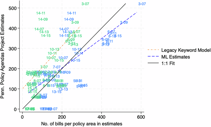
There is a stronger correlation between Machine Learning estimates and the Pennsylvania Policy Database Project than the legacy keyword model. Note: Estimates are labeled with the major topic number (see column 1 of Table 7 and the last two digits of the year.
In terms of reliability, methods designed to evaluate multi-label classification schemes26 show the machine learning estimates perform well. The average ranking loss is 0.11 (0.00 would be perfect, 0.50 would be near chance), which is slightly more ranking loss than the human coder exercise, but that is to be expected because of the measurement error aligning the codebooks. The top-K agreement between the model estimates and PPDP in Table 8 shows at K = 3 there is 70 percent agreement. So by considering three guesses per bill, the machine learning method produces a reasonable facsimile of what a human coder can be expected to produce. There also appears to be diminishing returns to the Top-K agreement near 90 percent. This reveals just how difficult this task may be, that even with many guesses it may not be reasonable to generate complete agreement.
Table 8 Top-K agreement of model estimates and Pennsylvania codes (n=1,000).