Learning quantum states of continuous-variable systems

Trace distance

The trace distance between two quantum states ρ1 and ρ2 is defined as

$${d}_{{\rm{tr}}}(\;{\rho }_{1},{\rho }_{2}):=\frac{1}{2}\|{\rho }_{1}-{\rho }_{2}\|_{1},$$

(11)

where \(\|A\|_{1}:={\rm{Tr}}\sqrt{{A}^{\dagger }A}\) denotes the trace norm. The trace distance is considered the most meaningful notion of distance between two states because of its operational meaning in terms of the optimal probability of discriminating between two states having access to a single copy of the state (Holevo–Helstrom theorem9,10). Consequently, in quantum information theory, the error in approximating a state is typically quantified using the trace distance.

Quantum-state tomography

In this section, we formulate precisely the problem of quantum-state tomography1, which forms the basis of our investigation. The basic set-up is depicted in Fig. 4.

Problem 7

(Quantum-state tomography) Let \({\mathcal{S}}\) be a set of quantum states. Consider ε, δ ∈ (0, 1) and \(N\in {\mathbb{N}}\). Let \(\rho \in {\mathcal{S}}\) be an unknown quantum state. Given access to N copies of ρ, the goal is to provide a classical description of a quantum state \(\tilde{\rho }\) such that

$$\Pr \left[{d}_{{\rm{tr}}}(\;\tilde{\rho },\rho )\le \varepsilon \right]\ge 1-\delta .$$

(12)

That is, with a probability ≥1 − δ, the trace distance between \(\tilde{\rho }\) and ρ is at most ε. Here ε is called the trace-distance error, and δ is called the failure probability.

The sample complexity, the time complexity and the memory complexity in the tomography of states in \({\mathcal{S}}\) are defined as the minimum number of copies N, the minimum amount of classical and quantum computation time, and the minimum amount of classical memory, respectively, required to solve Problem 7 with trace-distance error ε and failure probability δ. Note that the time complexity is always an upper bound on the memory complexity and the sample complexity.

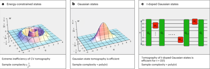
One can think of \({\mathcal{S}}\) as a specific subset of the entire set of n-qubit states (for example, pure states, r-rank states and stabilizer states) or n-mode states (for example, energy-constrained states, moment-constrained states, Gaussian states and t-doped Gaussian states). By definition, tomography is deemed efficient if the sample, time and memory complexities scale polynomially in n; otherwise, it is deemed inefficient. For example, in our work, we prove that the tomography of energy-constrained states is (extremely) inefficient. By contrast, the tomography of Gaussian states is efficient, whereas the tomography of t-doped Gaussian states is efficient for small t and inefficient for large t.

CV systems

In this section, we provide a concise overview of quantum information with CV systems7. A CV system is a quantum system associated with the Hilbert space \({L}^{2}({{\mathbb{R}}}^{n})\) of all square-integrable complex-valued functions over \({{\mathbb{R}}}^{n}\), which models n modes of electromagnetic radiation with definite frequency and polarization. A quantum state in \({L}^{2}({{\mathbb{R}}}^{n})\) is called an n-mode state, and a unitary operator in \({L}^{2}({{\mathbb{R}}}^{n})\) is called an n-mode unitary. The quadrature vector is defined as

$$\hat{{\bf{R}}}:={({\hat{x}}_{1},{\hat{p}}_{1},\ldots ,{\hat{x}}_{n},{\hat{p}}_{n})}^{\top },$$

(13)

where \({\hat{x}}_{j}\) and \({\hat{p}}_{j}\) are the well-known position and momentum operators of the jth mode, collectively called quadratures. Let us proceed with the definitions of a Gaussian unitary and a Gaussian state.

Definition 8

(Gaussian unitary) An n-mode unitary is Gaussian if it is the composition of unitaries generated by quadratic Hamiltonians \(\hat{H}\) in the quadrature vector

$$\hat{H}:=\frac{1}{2}{(\hat{{\bf{R}}}-{\bf{m}})}^{\top }h(\hat{{\bf{R}}}-{\bf{m}}),$$

(14)

for some symmetric matrix \(h\in {{\mathbb{R}}}^{2n,2n}\) and some vector \({\bf{m}}\in {{\mathbb{R}}}^{2n}\).

Definition 9

(Gaussian state) An n-mode state ρ is Gaussian if it can be written as a Gibbs state of a quadratic Hamiltonian \(\hat{H}\) of the form in equation (14) with h being positive definite. The Gibbs states associated with the Hamiltonian \(\hat{H}\) are given by

$$\rho ={\left(\frac{{e}^{-\beta \hat{H}}}{{\rm{Tr}}[\operatorname{e}^{-\beta \hat{H}}]}\right)}_{\beta \in [0,\infty ]},$$

(15)

where the parameter β is the inverse temperature.

This definition includes also the pathological cases where both β and certain terms of H diverge (for example, this is the case for tensor products between pure Gaussian states and mixed Gaussian states). An example of a Gaussian state vector is the vacuum, denoted as \({\left\vert 0\right\rangle }^{\otimes n}\). Any pure n-mode Gaussian state vector can be written as a Gaussian unitary G applied to the vacuum:

$$\left\vert \psi \right\rangle =G{\left\vert 0\right\rangle }^{\otimes n}.$$

(16)

A Gaussian state ρ is uniquely identified by its first moment m(ρ) and covariance matrix V(ρ). By definition, the first moment and the covariance matrix of an n-mode state ρ are given by

$$\begin{aligned}{\bf{m}}(\;\rho )&:={\rm{Tr}}\left[\hat{{\bf{R}}}\,\rho \right],\\ V(\;\rho )&:={\rm{Tr}}\left[\left\{(\hat{{\bf{R}}}-{\bf{m}}(\;\rho )),{(\hat{{\bf{R}}}-{\bf{m}}(\;\rho ))}^{\top }\right\}\rho \right],\end{aligned}$$

(17)

where \(\{\hat{A},\hat{B}\}:=\hat{A}\hat{B}+\hat{B}\hat{A}\) is the anti-commutator.

By definition, the energy of an n-mode state ρ is given by the expectation value \({\rm{Tr}}[{\hat{E}}_{n}\rho ]\) of the energy observable \({\hat{E}}_{n}:=\sum_{j = 1}^{n}({\hat{x}}_{j}^{2}+{\hat{p}}_{j}^{2})/2\), where it is assumed that each mode has a frequency of one7. It is important to note that energy is an extensive quantity, because for any single-mode state σ the energy of σ⊗n equals the energy of σ multiplied by n. Furthermore, the energy of an n-mode state is always greater than or equal to n/2, with the equality achieved only by the vacuum. The total number of photons can be defined in terms of the energy observable as

$${\hat{N}}_{n}:={\hat{E}}_{n}-\frac{n}{2}\hat{{\mathbb{1}}}.$$

(18)

Given \({\bf{k}}=({k}_{1},\ldots ,{k}_{n})\in {{\mathbb{N}}}^{n}\), let us denote as

$$\left\vert {\bf{k}}\right\rangle =\left\vert {k}_{1}\right\rangle \otimes \cdots \otimes \left\vert {k}_{n}\right\rangle$$

(19)

the n-mode Fock state vector7. The total number of photons is diagonal in the Fock basis as

$${\hat{N}}_{n}=\sum _{{\bf{k}}\in {{\mathbb{N}}}^{n}}\|{\bf{k}}\|_{1}\left\vert {\bf{k}}\right\rangle \left\langle {\bf{k}}\right\vert ,$$

(20)

where \(\|{\bf{k}}\|_{1}:=\sum_{i = 1}^{n}{k}_{i}\).

Effective dimension and rank of energy-constrained states

In this section, we show that energy-constrained states can be approximated well by finite-dimensional states with low rank, as anticipated above in equation (3). Further technical details regarding the findings presented in this section can be found in Supplementary Information.

Let ρ be an n-mode state with total number of photons satisfying the energy constraint

$${\rm{Tr}}[\;\rho {\hat{N}}_{n}]\le nE,$$

(21)

where E ≥ 0. Given \(M\in {\mathbb{N}}\), let \({{\mathcal{H}}}_{M}\) be the subspace spanned by all the n-mode Fock states with total number of photons not exceeding M, and let ΠM be the projector onto this space.

Let us begin by analysing the effective dimension of the set of energy-constrained states. The trace distance between the energy-constrained state ρ and its projection ρM onto \({{\mathcal{H}}}_{M}\), that is,

$${\rho }_{M}:=\frac{{\varPi }_{M}\rho {\varPi }_{M}}{\operatorname{Tr}[{\varPi }_{M}\rho ]},$$

(22)

can be upper bounded as follows:

$${d}_{{\rm{tr}}}(\;\rho ,{\rho }_{M})\mathop{\le }\limits^{({\rm{i}})}\sqrt{{\rm{Tr}}[({\mathbb{1}}-{\Pi }_{M})\rho ]}\mathop{\le }\limits^{({\rm{ii}})}\sqrt{\frac{{\rm{Tr}}[{\hat{N}}_{n}\rho ]}{M}}\le \sqrt{\frac{nE}{M}},$$

(23)

where in (i) we have employed the gentle measurement lemma52 and in (ii) we used the simple operator inequality \({\mathbb{1}}-{\varPi }_{M}\le {\hat{N}}_{n}/M\). Consequently, by setting M1 := ⌈nE/ε2⌉, it follows that the projection \({\rho }_{{M}_{1}}\) is ε-close to ρ in trace distance. Moreover, the dimension of \({{\mathcal{H}}}_{{M}_{1}}\) can be upper bounded as

$$\dim {{\mathcal{H}}}_{{M}_{1}}=\left(\begin{array}{c}n+{M}_{1}\\ n\end{array}\right)\le {\left(\frac{\mathrm{e}(n+{M}_{1})}{n}\right)}^{n}=O\left(\frac{{(\mathrm{e}E\;)}^{n}}{{\varepsilon }^{2n}}\right),$$

(24)

where e denotes Euler’s number. Hence, we conclude that any energy-constrained state ρ can be approximated, up to trace-distance error ϵ, by its projection \({\rho }_{{M}_{1}}\) onto the subspace \({{\mathcal{H}}}_{{M}_{1}}\), which has a finite dimension of \(O\left({(\mathrm{e}E)}^{n}/{\varepsilon }^{2n}\right)\).

Now, let us analyse the effective rank of the energy-constrained state ρ. We say that ρ has effective rank r if it is ε-close to a state with rank r. Let us consider the spectral decomposition

$$\rho =\sum_{i=1}^{\infty }{p}_{i}^{\downarrow }{\psi }_{i},$$

(25)

where the eigenvalues \({({p}_{i}^{\downarrow })}_{i}\) are not increasing in i. To estimate the effective rank, let us choose an integer r such that

$$\sum_{i=r+1}^{\infty }{p}_{i}^{\downarrow }\le \varepsilon ,$$

(26)

which guarantees that the r-rank state \({\rho }^{(r)}\propto \sum_{i = 1}^{r}{p}_{i}^{\downarrow }{\psi }_{i}\) is O(ε)-close to ρ. The infinite-dimensional Schur–Horn theorem (Proposition 6.4 in ref. 53) implies that for any r-rank projector Π,

$$\sum_{i=r+1}^{\infty }{p}_{i}^{\downarrow }\le {\rm{Tr}}[({\mathbb{1}}-\varPi )\rho ].$$

(27)

Moreover, by setting M2 := ⌈nE/ε⌉, the projector \({\varPi }_{{M}_{2}}\) is an O((eE)n/ϵn)-rank projector satisfying

$${\rm{Tr}}[({\mathbb{1}}-{\varPi }_{{M}_{2}})\rho ]\le \frac{{\rm{Tr}}[{\hat{N}}_{n}\rho ]}{{M}_{2}}\le \frac{nE}{M}\le \varepsilon ,$$

(28)

where we have employed the same inequalities used in equations (23) and (24). Hence, by setting \(\varPi ={\varPi }_{{M}_{2}}\), we deduce that ρ is ε-close to a state ρ(r) having rank

$$r=O\left({(\mathrm{e}E\;)}^{n}/{\varepsilon }^{n}\right).$$

(29)

Finally, by exploiting the gentle measurement lemma52 and triangle inequality, one can easily show that the projection of ρ(r) onto \({{\mathcal{H}}}_{{M}_{1}}\) is still O(ε)-close to ρ. Consequently, we conclude that any energy-constrained state can be approximated, up to trace-distance error ε, by a D-dimensional state with rank r such that

$$\begin{aligned}D&=O\left({(\mathrm{e}E\;)}^{n}/{\varepsilon }^{2n}\right),\\ r&=O\left({(\mathrm{e}E\;)}^{n}/{\varepsilon }^{n}\right).\end{aligned}$$

(30)

Based on these observations, we devised a simple tomography algorithm for energy-constrained states. The first step involves performing the two-outcome measurement \(({\varPi }_{{M}_{1}},{\mathbb{1}}-{\varPi }_{{M}_{1}})\) and discarding the post-outcome state associated with \({\mathbb{1}}-{\varPi }_{{M}_{1}}\). This step transforms the unknown state ρ into the state \({\rho }_{{M}_{1}}\) with high probability. The state \({\rho }_{{M}_{1}}\) has two key properties: (1) It resides in the finite-dimensional subspace \({{\mathcal{H}}}_{{M}_{1}}\) of dimension \(D=O\left({(\mathrm{e}E)}^{n}/{\varepsilon }^{2n}\right)\). (2) It is O(ε)-close to a state residing in \({{\mathcal{H}}}_{{M}_{1}}\) with rank r = O((eE)n/ϵn). The second step involves performing the tomography algorithm of ref. 54 designed for D-dimensional state with rank r, which has a sample complexity of O(Dr). Importantly, this algorithm remains effective even if the unknown state, which is promised to reside in a given D-dimensional Hilbert space, has rank strictly larger than r, as long as it is O(ε)-close to a r-rank state within the same Hilbert space54. We, thus, conclude that the sample complexity in the tomography of energy-constrained states is upper bounded by O(Dr) = O((eE)2n/ϵ3n). Analogously, by exploiting that the sample complexity in the tomography of D-dimensional pure states is O(D) (refs. 1,12,13,14), we can show that the sample complexity in the tomography of energy-constrained pure states is upper bounded by O(D) = O((eE)n/ϵ2n).

For completeness, let us mention that the proof of the lower bounds on the sample complexity in the tomography of energy-constrained states, as presented in Theorems 1 and 2, primarily relies on epsilon-net tools55, like the qudit systems tackled in refs. 12,54. Detailed proofs of these results can be found in Supplementary Information.

Bounds on the trace distance between Gaussian states

In this section, we address the question: If we know with a certain precision the first moment and the covariance matrix of an unknown Gaussian state, what is the resulting trace-distance error that we make on the state?

Let us formalize the problem. Let us consider a Gaussian state ρ1 and assume that we have an approximation of its first moment m(ρ1) and an approximation of its covariance matrix V(ρ1). For example, these approximations may be retrieved through homodyne detection on many copies of ρ1. We can then consider the Gaussian state ρ2 with first moment and covariance matrix equal to such approximations: m(ρ2) and V(ρ2) are, thus, the approximations of m(ρ1) and V(ρ1), respectively. The errors incurred in these approximations are naturally measured by the norm distances ∥m(ρ1) − m(ρ2)∥ and ∥V(ρ1) − V(ρ2)∥, respectively, where ∥ ⋅ ∥ denotes some norm. Now, a natural question arises: given an error ε in the approximations of the first moment and covariance matrix, what is the error incurred in the approximation of ρ1? The most meaningful way to measure such an error is given by the trace distance dtr(ρ1, ρ2) (refs. 9,10). Hence, the question becomes the following. If it holds that

$$\begin{aligned}\| {\bf{m}}(\;{\rho }_{1})-{\bf{m}}(\;{\rho }_{2})\| &=O(\varepsilon ),\\ \| V(\;{\rho }_{1})-V(\;{\rho }_{2})\| &=O(\varepsilon ),\end{aligned}$$

(31)

what can we say about the trace distance dtr(ρ1, ρ2)? Thanks to Theorems 10 and 11, we can answer this question. The trace distance dtr(ρ1, ρ2) is at most \(O(\sqrt{\varepsilon })\) and at least Ω(ε).

This motivates the problem of finding upper and lower bounds on the trace distance between Gaussian states in terms of the norm distance of their first moments and covariance matrices. Now, we present our bounds, which are technical tools of independent interest.

Theorem 10, proven in Supplementary Information, gives our upper bound on the trace distance between Gaussian states.

Theorem 10

(Upper bound on the distance between Gaussian states) Let ρ1 and ρ2 be n-mode Gaussian states satisfying the energy constraint \({\rm{Tr}}[{\hat{N}}_{n}{\rho }_{1}],{\rm{Tr}}[{\hat{N}}_{n}{\rho }_{2}]\le N\). Then,

$$\begin{aligned}{d}_{{\rm{tr}}}({\rho }_{1},{\rho }_{2})&\le f(N)\bigg(\|{\bf{m}}(\;{\rho }_{1})-{\bf{m}}(\;{\rho }_{2})\| +\sqrt{2}\sqrt{\|V(\;{\rho }_{1})-V(\;{\rho }_{2}){\|}_{1}}\bigg),\end{aligned}$$

(32)

where \(f(N):=\frac{1}{\sqrt{2}}\big(\sqrt{N}+\sqrt{N+1}\big)\). Here \(\|{\bf{m}}\|:=\sqrt{{{\bf{m}}}^{\top }{\bf{m}}}\) and ∥ ⋅ ∥1 denote the Euclidean norm and the trace norm, respectively.

The above theorem turns out to be crucial for proving the upper bound on the sample complexity in the tomography of Gaussian states provided in Theorem 4.

One might believe that proving Theorem 10 would be straightforward by bounding the trace distance using the closed formula for the fidelity between Gaussian states56. However, this approach turns out to be highly non-trivial due to the complexity of such a fidelity formula56, which makes it challenging to derive a bound based on the norm distance between the first moments and covariance matrices. Instead, our proof directly addresses the trace distance without relying on fidelity and involves a meticulous analysis based on the energy-constrained diamond norm57.

The following theorem, proven in Supplementary Information, establishes our lower bound on the trace distance between Gaussian states.

Theorem 11

(Lower bound on the distance between Gaussian states) Let ρ1 and ρ2 be n-mode Gaussian states satisfying the energy constraint \({\rm{Tr}}[{\hat{E}}_{n}{\rho }_{1}],{\rm{Tr}}[{\hat{E}}_{n}{\rho }_{2}]\le E\). Then,

$$\begin{aligned}{d}_{{\rm{tr}}}(\;{\rho }_{1},{\rho }_{2})&\ge\frac{1}{200}\min \left\{1,\frac{\parallel {\bf{m}}(\;{\rho }_{1})-{\bf{m}}(\;{\rho }_{2})\parallel }{\sqrt{4E+1}}\right\},\\ {d}_{{\rm{tr}}}(\;{\rho }_{1},{\rho }_{2})&\ge\frac{1}{200}\min \left\{1,\frac{\parallel V(\;{\rho }_{2})-V(\;{\rho }_{1}){\parallel }_{2}}{4E+1}\right\},\end{aligned}$$

(33)

where \(\|{\bf{m}}\|:=\sqrt{{{\bf{m}}}^{\top }{\bf{m}}}\) and \(\parallel V{\parallel }_{2}:=\sqrt{{\rm{Tr}}[{V}^{\top }V]}\) denote the Euclidean norm and the Hilbert–Schmidt norm, respectively.

The proof of this theorem relies heavily on state-of-the-art bounds recently established for Gaussian probability distributions58.

Theorems 10 and 11 allow us to answer the question posed at the beginning of this section. Indeed, these theorems imply that, if we know with error ε the first moment and the covariance matrix of an unknown Gaussian state, the resulting trace-distance error that we make on the state is at most \(O(\sqrt{\varepsilon })\) and at least Ω(ε). In particular, this proves Theorem 3.

The trace-distance bound of Theorem 10 can be improved by assuming one of the Gaussian states to be pure, as we detail in the following theorem, which is proven in the Supplementary Information.

Theorem 12

(Improved bound for pure states) Let ψ be a pure n-mode Gaussian state and let ρ be an n-mode (possibly non-Gaussian) state satisfying the energy constraints \({\rm{Tr}}[\psi {\hat{E}}_{n}],{\rm{Tr}}[\rho {\hat{E}}_{n}]\le E\). Then

$${d}_{{\rm{tr}}}(\;\rho ,\psi )\le \sqrt{E}\sqrt{2\|{\bf{m}}(\;\rho )-{\bf{m}}(\psi ){\|}^{2}+\|V(\;\rho )-V(\psi ){\|}_{\infty }},$$

(34)

where \(\|{\bf{m}}\|:=\sqrt{{{\bf{m}}}^{\top }{\bf{m}}}\) and ∥ ⋅ ∥∞ denote the Euclidean norm and the operator norm, respectively.

By exploiting this improved bound, we show in Supplementary Information that the tomography of pure Gaussian states can be achieved using O(n5E3/ϵ4) copies of the state. This represents an improvement over the mixed-state scenario considered in Theorem 4.

Moreover, the bound in Theorem 12 can be useful for quantum-state certification15, as we briefly detail now. Suppose one aims to prepare a pure Gaussian state ψ with known first moment and covariance matrix. In a noisy experimental set-up, however, an unknown state ρ is effectively prepared. By accurately estimating the first two moments of ρ (which can be done efficiently, as shown in Supplementary Information), one can estimate the right-hand side of equation (34), which provides an upper bound on the trace distance between the target state ψ and the noisy state ρ, thereby providing a measure of the precision of the quantum device. Consequently, the device can be adjusted to minimize the error in state preparation.