
Theoretical formulation
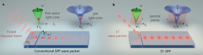
The conceptual formulation of ST-SPPs is best understood by visualizing their spectral representation on the surface of the light-cone. For (2 + 1)D pulsed optical fields restricted to one transverse dimension x in addition to the axial dimension z, the light-cone is the geometric representation of the dispersion relationship involving the transverse wave number kx (or spatial frequency), the longitudinal wave number kz, and the temporal frequency ω. In free space, the light-cone is \({k}_{x}^{2}+{k}_{z}^{2}={(\frac{\omega }{c})}^{2}\), and that for an SPP at a metal-dielectric interface is \({k}_{x}^{2}+{k}_{z}^{2}={k}_{{{\rm{SPP}}}}^{2}(\omega )\); where c is the speed of light in vacuum, \({k}_{{{\rm{SPP}}}}=\frac{\omega }{c}\sqrt{\frac{{\epsilon }_{{{\rm{m}}}}{\epsilon }_{{{\rm{d}}}}}{{\epsilon }_{{{\rm{m}}}}+{\epsilon }_{{{\rm{d}}}}}}\), and ϵm and ϵd are the relative permittivities of the metal and dielectric, respectively (Fig. 1a). In free space, where a (2 + 1)D pulsed beam (or wave packet) takes the form of a light-sheet that is uniform along y and localized along x, its spectral support is a two-dimensional (2D) region on the surface of the free-space light-cone (Fig. 1a). Such a light-sheet undergoes diffractive spreading with free propagation. A conventional SPP wave packet is a (2 + 1)D surface wave with finite transverse-spatial extent along x in addition to surface localization along y, whose spectral support in turn corresponds to a 2D region on the surface of the SPP light-cone (Fig. 1a)35,48. This conventional SPP wave packet undergoes both diffractive spreading in space and dispersive spreading in time.
Ideal STWPs are pulsed beams that propagate rigidly in linear media without diffraction or dispersion, and whose propagation characteristics can be tuned largely independently of the material parameters23,28. Rather than the 2D spectral support on the free-space light-cone associated with conventional pulsed light sheets, the spatiotemporal spectrum of an STWP is restricted to a 1D curve (a conic section) at the intersection of the light-cone with a plane that is parallel to the kx-axis and makes an angle θ with the kz-axis (Fig. 1b)28. This plane, \(\omega -{\omega }_{{{\rm{o}}}}=({k}_{z}-{k}_{{{\rm{o}}}})c\,\tan \theta\), results in a straight-line spectral projection onto the \(({k}_{z},\frac{\omega }{c})\)-plane, which indicates a fixed group velocity \(\widetilde{v}=c\,\tan \theta\) and the absence of dispersion to all orders49; here ωo is a fixed carrier frequency, and \({k}_{{{\rm{o}}}}=\frac{{\omega }_{{{\rm{o}}}}}{c}\) is its associated wave number. Moreover, the one-to-one association between ω and ∣kx∣ guarantees diffraction-free propagation of the time-averaged intensity23. Similarly for ST-SPPs, their spectral support as shown in Fig. 1b is also a 1D curve at the intersection of the SPP light-cone with the plane \(\omega -{\omega }_{{{\rm{o}}}}=({k}_{z}-{k}_{{{\rm{o}}}}^{{\prime} }){\widetilde{v}}_{{{\rm{SPP}}}}\tan \theta\), where \({\widetilde{v}}_{{{\rm{SPP}}}}\) is the group velocity of a plane-wave pulsed SPP at ω = ωo, and \({k}_{{{\rm{o}}}}^{{\prime} }\) is the SPP wave number at ωo35. The spectral projection onto the (\({k}_{z},\frac{\omega }{c}\))-plane for the ST-SPP is also a straight line, indicating that – in addition to being diffraction-free – ST-SPPs propagate dispersion-free at a group velocity \(\widetilde{v}={\widetilde{v}}_{{{\rm{SPP}}}}\tan \theta\) despite the intrinsic GVD associated with freely propagating SPPs (Fig. 1b)35.
We show in Fig. 2 (first row) the spectral support for a conventional SPP wave packet on the SPP light-cone (Fig. 2a), its spectral projections onto the \(({k}_{x},\frac{\omega }{c})\) and \(({k}_{z},\frac{\omega }{c})\) planes (Fig. 2b, c), along with the out-of-plane field profile (Fig. 2d). We assume a separable Gaussian spectrum in space and time, and take into account the temporal bandwidth Δ λ ≈ 110 nm (FWHM) utilized in our experiments (Methods). Crucially, the phase front for this conventional SPP wave packet is orthogonal to the propagation axis z (Fig. 2d).
Fig. 2: Spectral representation of SPPs and ST-SPPs.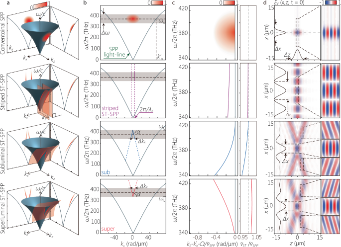
The first row corresponds to a conventional SPP wave packet with Δx = 9 μm; the second to a striped ST-SPP with λx = 10 μm; the third to a subluminal ST-SPP with Δx = 5 μm; and the fourth to a superluminal ST-SPP with Δx = 5 μm. (a) The spectral support on the surface of the SPP light-cone \({k}_{x}^{2}+{k}_{z}^{2}={k}_{{{\rm{SPP}}}}^{2}\) in \(({k}_{x},{k}_{z},\frac{\omega }{c})\)-space (shown in red). b The projection of the spectral support in a onto the \(({k}_{x},\frac{\omega }{c})\)-plane. This spectral projection is invariant upon coupling the field from free space to the metal-dielectric interface (as a consequence of conservation of energy and transverse momentum). The gray band corresponds to the bandwidth Δω of the laser pulse used in our experiments, and the dashed horizontal line is at \(\frac{{\omega }_{{{\rm{o}}}}}{2\pi }\approx 375\) THz (λo ≈ 800 nm in free space). c The spectral projection onto the \(({k}_{z},\frac{\omega }{c})\)-plane after implementing \({k}_{z}\to {k}_{z}-{k}_{{{\rm{o}}}}^{{\prime} }-\frac{\Omega }{{\widetilde{v}}_{{{\rm{SPP}}}}}\) for clarity, where Ω = ω−ωo. The panel to the right shows the group velocity of the wave packet \(\widetilde{v}=\frac{d\omega }{d{k}_{z}}\) normalized to \({\widetilde{v}}_{{{\rm{SPP}}}}\). The spectral range on the vertical axis corresponds to the bandwidth of the laser pulse. d The calculated out-of-plane real part of the field distribution Ey(x, y, z; t) at y = 0 and t = 0 (Methods). The black curves on the left and bottom are cross-sections at z = 0 and x = 0, respectively. The right panels show magnified views of the dashed squares in the left panel, highlighting the structure of the phase fronts.
Producing an ideal ST-SPP with a bandwidth Δ λ = 110 nm is prohibitive, as can be understood by considering a so-called ‘striped ST-SPP’ whose spatial profile results simply from the interference of a pair of plane waves with fixed spatial frequencies ± kx (i.e., the field takes the transverse form \(\cos {k}_{x}x\))42. Consequently, a striped ST-SPP is separable with respect to space and time, and it thus does not offer the possibility of tuning the group velocity (indeed, its group velocity is \(\widetilde{v}\approx {\widetilde{v}}_{{{\rm{SPP}}}}\); Methods). We plot in Fig. 2a–c (second row) the spectral support for a striped ST-SPP, which is the intersection of iso-∣kx∣ planes with the SPP light-cone. The out-of-plane field is separable, extended and periodic along x (with period λx ≡ 2π/kx = 10 μm), and its phase front is orthogonal to the z-axis, leading to a lattice-like spatial distribution at any instant t (Fig. 2d).
A broadband ST-SPP is composed of a multiplicity of cosine SPPs with different kx, each of which is associated with a prescribed ω, such that kz is maintained in a linear relationship with ω. However, maintaining this linear relationship between kz and ω over a large temporal bandwidth Δ ω is prohibitive for SPPs because the curvature of the SPP light-line dictates a large accompanying spatial bandwidth Δ kx. Indeed, even if \(\widetilde{v}\) it remains within 1% of \({\widetilde{v}}_{{{\rm{SPP}}}}\), we still need\(\frac{\Delta {k}_{x}}{{k}_{{{\rm{o}}}}}\approx 0.23\) (with the parameters used in our experiments below) to maintain the spatiotemporal spectrum of an ideal ST-SPP over the large bandwidth Δ λ ≈ 110 nm used here. Because our experimental scheme conserves the spatial bandwidth Δ kx from free space to the surface-bound field, a large numerical aperture is required. We define \({k}_{x}(\lambda )=\frac{2\pi }{\lambda }\sin \{\varphi (\lambda )\}=\frac{2\pi }{{\lambda }_{x}}\) in free space, where λ is the free-space wavelength, φ(λ) is the its propagation angle with the z-axis, and \({\lambda }_{x}=\lambda /\sin \varphi (\lambda )\) is the transverse period of the field along x. Our system is limited to a maximum angular acceptance \({\varphi }_{\max }\approx \pm {5}^{\circ }\), a numerical aperture (NA) of ≈ 0.09, which restricts the minimum spatial feature size to ≈ 9 μm which falls considerably short of the requirement for an ideal ST-SPP over Δ λ = 110 nm. To address this challenge, we have implemented a compromise regarding the structure of the realized ST-SPP with respect to an ideal ST-SPP: (1) we maintain the one-to-one correspondence between ∣kx∣ and ω that is necessary for diffraction-free propagation; (2) we maintain control over the group velocity \(\widetilde{v}\) of the ST-SPP away from that for a conventional SPP \({\widetilde{v}}_{{{\rm{SPP}}}}\) in both the subluminal (\(\widetilde{v} < {\widetilde{v}}_{{{\rm{SPP}}}}\)) and superluminal (\(\widetilde{v} > {\widetilde{v}}_{{{\rm{SPP}}}}\)) regimes; however (3) we allow the spectral projection onto the \(({k}_{z},\frac{\omega }{c})\)-plane to be curved such that it lies in the \(({k}_{z},\frac{\omega }{c})\)-plane between the SPP light-line and the linear spectral projection for an ideal ST-SPP (Fig. 2c). Consequently, we can operate with the available system NA, but at the cost of vouchsafing the complete elimination of GVD. This is a minimal disadvantage in light of the short SPP propagation distance limited by ohmic losses.
The spectral support of the realized ST-SPP is still a 1D curve on the surface of the SPP light-cone, but this curve results from the intersection of the SPP light-cone with a curved planar surface (rather than a plane) designed to yield a V-shaped spectral projection onto the \(({k}_{x},\frac{\omega }{c})\)-plane50. For a subluminal ST-SPP (\(\widetilde{v} < {\widetilde{v}}_{{{\rm{SPP}}}}\)), this projection takes the form \(\omega -{\omega }_{{{\rm{U}}}}=c| {k}_{x}| \tan \alpha\), where \({\omega }_{{{\rm{U}}}}={\omega }_{{{\rm{o}}}}+\frac{\Delta \omega }{2}\) is the maximum frequency, ω < ωU, α is the angle with the kx-axis, and \(\tan \alpha < 0\). For a superluminal ST-SPP (\(\widetilde{v} > {\widetilde{v}}_{{{\rm{SPP}}}}\)), we have \(\omega -{\omega }_{{{\rm{L}}}}=c| {k}_{x}| \tan \alpha\), where \({\omega }_{{{\rm{L}}}}={\omega }_{{{\rm{o}}}}-\frac{\Delta \omega }{2}\) is the minimum frequency, ω > ωL, and \(\tan \alpha > 0\). In both cases, ωo is the central frequency, so that \({\omega }_{{{\rm{o}}}}-\frac{\Delta \omega }{2} < \omega < {\omega }_{{{\rm{o}}}}+\frac{\Delta \omega }{2}\). This curved surface remains parallel to the kx-axis, but its projection onto the \(({k}_{z},\frac{\omega }{c})\)-plane is no longer a straight line and is instead a curve that remains closer to the SPP light-line than in the case of the ideal ST-SPP (to remain within the system NA). The analytical relationship between ST-SPP group velocity \(\widetilde{v}\) and the angle α is derived in Methods. The GVD coefficient for a conventional SPP wave packet in this case is 2.5 × 10³ fs2/mm, and is 2.5 × 10³, 2.3 × 10², and 2.0 × 10² fs2/mm for a striped ST-SPP (with λx = 10 μm), a subluminal ST-SPP (with α = −64.5∘), and a superluminal ST-SPP (with α = 64. 5°), respectively.
We plot in Fig. 2 the spectral representation for the subluminal ST-SPP (third row) and the superluminal ST-SPP (fourth row). Of particular interest is the spatial profile of the out-of-plane field for both ST-SPPs, which is no longer separable as a result of the non-separability of their spatiotemporal spectra. Instead, we observe an X-shaped profile reminiscent of free-space STWPs49,51. Crucially, the direction of the phase fronts varies across the wave front. In the vicinity of the center x = 0, the phase front is orthogonal to the propagation axis. However, along the branches of the X-shaped profile, the phase fronts are tilted with respect to the z-axis. Crucially, the sign of this phase-front tilt switches between the subluminal and superluminal regimes, and the magnitude of the tilt angle increases with the deviation of \(\widetilde{v}\) from \({\widetilde{v}}_{{{\rm{SPP}}}}\)52.
Experimental arrangement
We sketch in Fig. 3a the optical arrangement for synthesizing free-space STWPs, launching them into ST-SPPs on a metal-dielectric interface via scattering from a nano-slit, and observing the propagation of surface-bound ST-SPPs via spatially and temporally resolved two-photon fluorescence produced from the interference of the ST-SPP with a free-space reference pulse. We start with pulses from a Ti:sapphire laser oscillator of bandwidth Δ λ ≈ 110 nm (FWHM), center wavelength λo ≈ 800 nm, and a 10-fs transform-limited pulse duration (FWHM). However, the measured pulse width at the sample surface is Δ T ≈ 16 fs (FWHM) because of residual chirp in the optical system.
Fig. 3: Experimental arrangement for synthesizing, launching, and observing ST-SPPs.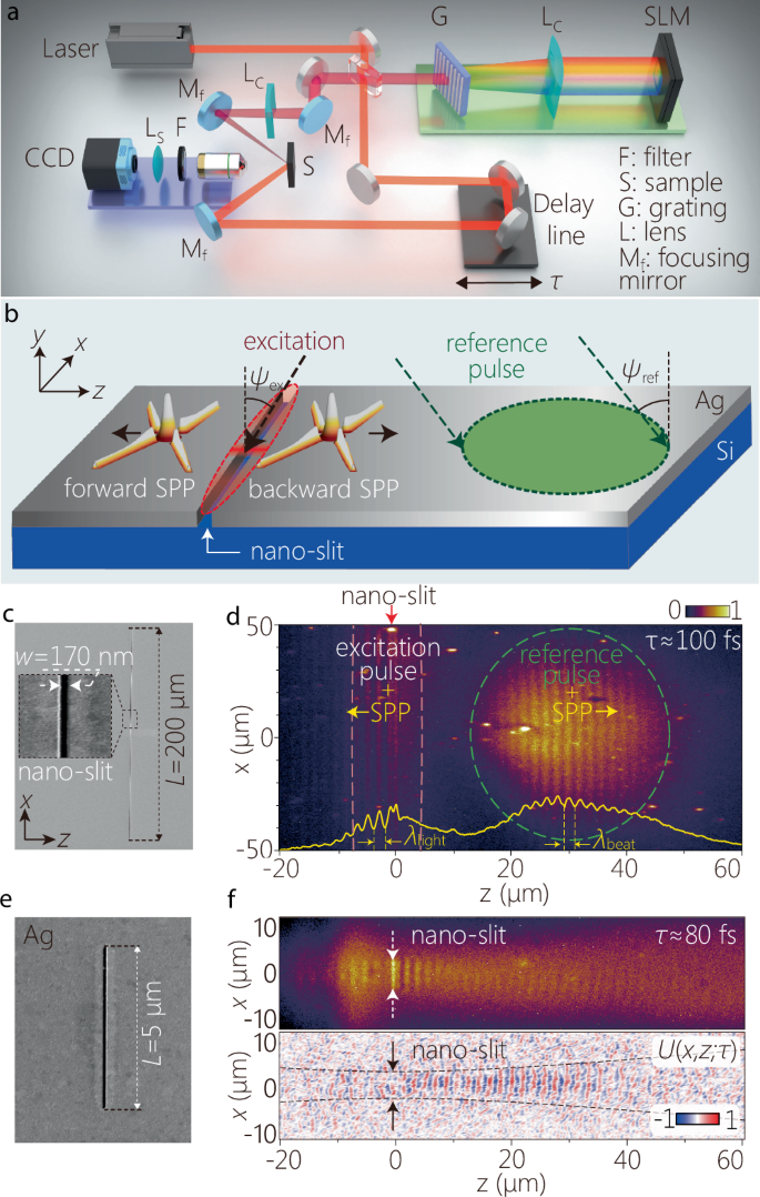
a Schematic of the setup for synthesizing free-space STWPs, launching them onto the sample, and imaging of the surface-bound field. b Schematic of the sample irradiation configuration. The STWP incidence angle is ψex = −45∘ to the surface normal, and the reference pulse incidence angle is ψref = 45∘. c SEM micrograph of the nano-slit milled into the Ag film. The inset shows a section of the nano-slit. d Two-photon fluorescence beat profile I(x, z; τ) at a fixed delay τ for a conventional SPP wave packet launched from the nano-slit. The yellow curve at the bottom is the axial profile I(z; τ) = ∫ dx I(x, z; τ) at a fixed τ. The red arrow at the top indicates the nano-slit location. Dashed orange lines enclose the irradiation area of the excitation, and the dashed green circle encloses that for the reference pulse. e SEM micrograph of the 5-μm-long nano-slit used to launch a conventional SPP wave packet of that width. f The two-photon fluorescence beat pattern (upper panel) after irradiating the nano-slit in (e), and the extracted field U(x, z; τ) (lower panel), both at fixed delay τ ≈ 80 fs (see Supplementary Movies 1 and 2). The dotted black curves correspond to the width of a Gaussian beam of width 5 μm (1/e2 full width of the intensity), and serve as a guide for the eye.
Synthesis of ST-SPPs
The STWPs are synthesized from the pulsed laser via spatiotemporal spectral phase modulation as established in refs. 28,49. The pulse spectrum is spatially resolved by a grating (300 lines/mm), the first diffraction order is selected and collimated using a cylindrical lens, which then impinges on a reflective, phase-only spatial light modulator (SLM); see Fig. 3a. This SLM imparts a 2D phase distribution to the incident wave front to deflect each wavelength λ by angles ± φ(λ) with respect to the z-axis, where \(\sin \{\varphi (\lambda )\}=\pm (1-\frac{\lambda }{{\lambda }_{{{\rm{c}}}}})\cot \alpha\). Here λc is the minimum (λ > λc) or the maximum (λ < λc) wavelength in the superluminal or subluminal regimes, respectively. The reflected phase-modulated wavefront is directed to a second grating identical to the first, whereupon the pulse is reconstituted to produce the STWP. For simplicity, the synthesis system in Fig. 3a is depicted as retro-reflecting from the SLM (whereupon the second grating coincides with the first); see Methods for details.
Sample preparation and launching ST-SPPs onto a metal-dielectric interface
The sample is a 100-nm-thick Ag film deposited on a silicon substrate. A crucial experimental challenge is to couple a broadband free-space STWP to a surface-bound ST-SPP at the metal-dielectric interface. We have recently examined theoretically an alternative approach to launching free-space STWPs into ST-SPPs that relies on scattering from a nano-slit in the metal surface (Fig. 3b)41. This coupling strategy retains a high efficiency over the bandwidth used here, and is thus preferable to conventional approaches for SPP coupling (e.g., gratings or evanescent prism-coupling) that modify the transverse wave number or do not operate over large bandwidths. Such a nano-slit conserves the transverse wave number \({k}_{x}^{{{\rm{free}}}}={k}_{x}^{{{\rm{SPP}}}}={k}_{x}\), where \({k}_{x}^{{{\rm{free}}}}\) and \({k}_{x}^{{{\rm{SPP}}}}\) are the transverse wave numbers for the free-space field and the launched SPP on either side of the nano-slit, respectively, so that the axial wave number is \({k}_{z}=\pm \sqrt{{k}_{{{\rm{SPP}}}}^{2}-{k}_{x}^{2}}\).
Two sets of 170-nm-wide, 100-nm-deep nano-slits were milled into the Ag film (Fig. 3c, e). One set of nano-slits has a lateral length of 200 μm and is used to launch ST-SPPs onto the Ag surface when illuminated with a free-space STWP (Fig. 3c). When illuminated with a conventional pulsed beam of large transverse extent along x, a conventional SPP wave packet is launched with a transverse width equal to that of the incident field (Fig. 3d). The second set of nano-slits has a reduced lateral length of 5 μm (Fig. 3e), and is used to launch conventional SPPs with a 5-μm-wide spatial profile (Fig. 3f). We have experimentally confirmed the efficacy of the nano-slit coupling methodology with striped ST-SPPs42, the spatiotemporally separable building blocks of ST-SPPs that comprise a single spatial frequency. Our results here confirm the theoretical predictions in ref. 41 regarding the broadband coupling of STWPs to ST-SPPs. Finally, the sample is coated by a 30-nm-thick dye-doped PMMA film to form a two-photon fluorescent layer.
Spatiotemporal characterization of the ST-SPPs
A portion of the initial laser pulse (20% by power) is split off to serve as a reference pulse, while the remainder (80%) is directed to the above-described STWP synthesis system (Fig. 3a). The synthesized STWP that excites the ST-SPP is incident obliquely at an angle ψex = −45∘ with respect to the sample normal, and is focused via a combination of spherical mirror and cylindrical lens onto the nano-slit, which launches it onto the sample surface (Fig. 3b; Methods)42. The incident free-space field is launched by the nano-slit in both the forward and backward directions53,54 (Fig. 3b). The reference pulse traverses an optical delay line τ and is then focused onto the metal surface away from the nano-slit to interact with the surface-bound SPP. The interference beat pattern of the SPP and the reference pulse excites two-photon fluorescence from the polymer layer55. Because we aim at detecting exclusively the interference of the reference pulse with the SPP, after eliminating any interference between the incident STWP excitation and the excited ST-SPP, we make use of the backward-coupled SPP (z > 0) rather than the stronger forward-coupled SPP (z < 0); see Fig. 3b.
Observation of SPPs and ST-SPPsTime-resolved measurements
We show in Fig. 3d the fluorescence profile of a conventional SPP wave packet with a large transverse spatial profile excited by irradiating the nano-slit in Fig. 3c with a conventional pump pulse after setting the SLM phase to 0 everywhere; i.e., φ(λ) = 0. The beat profile to the left of the nano-slit (z < 0) results from self-interference of the launched SPP and the incident free-space excitation, which is thus stationary and independent of τ because the reference pulse is not involved. The two-photon fluorescence beat profile to the right is delimited by the irradiation area of the reference pulse on the sample surface (green dashed circle; focal spot 30 × 60 μm2). The delay τ is adjusted to correspond to the propagating SPP wave packet reaching z ~ 30 μm. We define t as the time incurred by the surface-bound SPP (that travels at a group velocity \(\widetilde{v}\)) to propagate from the nano-slit to the observation location. The time t will be different from the free-space delay τ placed in the path of the focused reference pulse (that travels at a group velocity \(c/\sin {\psi }_{{{\rm{ref}}}}\) along the metal surface) to reach the same location and produce the interference beat pattern; see Methods for the conversion between the delay τ and the time t.
We are now in a position to compare the time-resolved measurements of conventional SPP wave packets and ST-SPPs. We first investigate a conventional SPP wave packet where the initial laser pulses are focused onto the metal surface at the location of a 5-μm-long nano-slit (Fig. 3e). A conventional SPP wave packet is thus launched at the metal surface with a flat intensity profile, 5-μm transverse spatial width, and 16-fs temporal pulse width. The recorded two-photon fluorescence beat profile resulting from the launched SPP interfering with the reference pulse (focused spot size 60 × 15 μm2) is shown in Fig. 3f. The intensity drops due to ohmic losses and diffractive spreading, and only a faint arc-shaped beat pattern is visible when the SPP wave packet reaches z ~ 40 μm. From this intensity profile we extract the SPP field distribution U(x, z; τ) plotted in the bottom panel of Fig. 3 f at fixed delay τ ≈ 80 fs (Methods); see Supplementary Movies 1 and 2.
In Fig. 4 we plot the experimentally recorded and the computed two-photon fluorescence beat profiles at a fixed delay τ (Methods) for a conventional SPP of width 5 μm (Fig. 4a,b); a striped ST-SPP with transverse period ≈ 10 μm (Fig. 4c,d); a subluminal ST-SPP with α = −64. 5∘ (Fig. 4e,f); and a superluminal ST-SPP with α = 64. 5∘ (Fig. 4g, h). The differences in the wave packet center position and the extent of the interference envelopes are attributed to uncertainties in the time origin, spatial inhomogeneity in the fluorescent film, and variations in the intensity distribution of the probe beam. Typical time-resolved measurements of ST-SPPs are provided in Supplementary Movies 3–6. Computed spatiotemporal profiles capture all the key features of their measured counterparts. Crucially, the different phase front structures predicted in Fig. 2d are clearly observable, as depicted in the insets of the corresponding panels in Fig. 4. Whereas the conventional SPP has a flat phase front orthogonal to the z-axis (Fig. 4a, b, and Fig. 2d, first row), the striped ST-SPP has a checkered lattice-like structure (Fig. 4c,d, and Fig. 2d, second row). The phase front for the subluminal ST-SPP away from its center is tilted with respect to the z-axis (Fig. 4e, f, and Fig. 2d, third row). The sign of this phase-front tilt is reversed for the superluminal ST-SPP (Fig. 4g, h, and Fig. 2d, fourth row). The remaining quantitative differences between the computed and measured profiles in Fig. 4 are attributed to the residual chirp in the laser pulses, additional chirp encumbered in the STWP synthesis system, and spectral dissipation at the metal surface.
Fig. 4: Time-resolved two-photon fluorescence beat profiles for SPPs and ST-SPPs.
a Measured two-photon fluorescence beat profiles I(x, z; τ) at a fixed delay τ produced by the interference of a conventional SPP wave packet (of transverse spatial width 5 μm) with the reference pulse. Inset is a contrast-adjusted magnified view of the area enclosed in the dashed white rectangle (10 × 16 μm2) to highlight the flat wave front. b Calculated profile I(x, z; τ) corresponding to the measurement in (a); see Methods. c, d Same as a, b but for a striped ST-SPP with λx ≈ 10 μm. e, f Same as a, b but for a subluminal ST-SPP; and g, h for a superluminal ST-SPP. The white dashed lines are guides for the eye representing the propagating wavefronts, and the insets highlight the tilted wave fronts at the edges of the ST-SPPs. All the two-photon fluorescence micrographs are acquired at a delay τ ≈ 75 fs. The time t listed at the bottom left of the calculated profiles is that needed for each SPP to reach z = 35 μm (Methods). The focused spot size of the reference pulse was ≈ 60 × 15 μm2 in (a–d), and ≈ 30 × 50 μm2 in (e–h).
We have thus confirmed that the nano-slit is capable of launching free-space STWPs onto the metal surface as ST-SPPs, and that our experimental configuration can capture the time-resolved structure of the surface-bound, propagating ST-SPPs. We proceed to utilize this capability to verify two key features of ST-SPPs: their diffraction-free propagation, and the controllability of their group velocity (\(\widetilde{v}\)) above and below that of a conventional SPP (\({\widetilde{v}}_{{{\rm{SPP}}}}\)).
Diffraction-free propagation of ST-SPPs
To verify the diffraction-free behavior of the ST-SPPs, we evaluated the intensity profiles I(x, z) = ∫ dτ∣Ubeat(x, z; τ)∣2 at different axial positions by time-integration of the extracted field profiles Ubeat(x, z; t) obtained by removing background intensity from the two-photon fluorescence beat profiles (Methods). We plot in Fig. 5 the time-averaged intensity profiles for the striped ST-SPP (Fig. 5a), the subluminal ST-SPP (Fig. 5b), and the superluminal ST-SPP (Fig. 5c). For each case, we plot the intensity profiles obtained after focusing the reference pulse at two different axial positions along the sample surface: at z ≈ 35 μm and z ≈ 85 μm measured from the location of the nano-slit.
Fig. 5: Diffraction-free propagation of ST-SPPs.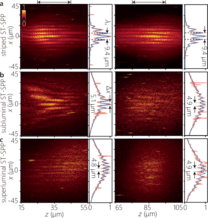
We plot the measured time-averaged intensity profiles for a a striped ST-SPP, b a subluminal ST-SPP, and c a superluminal ST-SPP. Time-averaged intensity profiles I(x, z; τ) are measured at two locations for the reference pulse. The left panel corresponds to the reference pulse focused near the nano-slit at 15 < z < 55 μm (with delay in the range τ ≈ 20 − 130 fs), and the right panel to the reference pulse focused away from it at 65 < z < 105 μm (τ ≈ 130−230 fs). The intensity profiles I(x) plotted to the right of each panel are obtained by axial integration I(x) = ∫ dz I(x, z) over the range identified by the black arrows on top (red curves), along with least-square fits (blue curves). The overall intensity distribution of the fluorescence profiles is affected by the irradiated region of the reference light. The Rayleigh ranges for the corresponding beam waists are 18.2 μm for the striped ST-SPP and 21 μm for the superluminal and subluminal ST-SPPs, respectively.
In contrast to a conventional SPP wave packet whose profile diffracts rapidly with propagation (Fig. 3f), the profiles of the ST-SPPs remain unchanged over the same propagation distance. In the case of the striped ST-SPP, this is to be expected because it contains only a single transverse wave number (i.e., an extended cosine wave profile). The limited transverse profile is a result of the narrow reference pulse irradiation spot utilized at the sample surface. The intensity profiles in Fig. 5a demonstrate that the striped ST-SPP maintains the same profile over a range of ≈ 5 × the Rayleigh range (zR ≈ 18.2 μm; Methods). The transverse profiles of the subluminal (Fig. 5b) and superluminal (Fig. 5c) ST-SPPs are also maintained over the distance examined, which is over ≈ 4 × Rayleigh lengths (the Rayleigh length is zR ≈ 21 μm). The reduced visibility in these time-averaged profiles compared to the time-resolved measurements in Fig. 4e,g is attributed to the integration over the full spatiotemporal field, which includes a broadband pedestal that partially obscures the localized structures.28,49 In all cases, the integrated cross-section along x plotted in the right panel is reasonably fitted by the (superposition) of Gaussian functions (representing the focused spot of the reference pulse) and the square of the sinusoidal-Gaussian function (representing the ST-SPP). The propagation distance here is limited by the ohmic losses. It is expected that the diffraction-free behavior extends significantly beyond 4zR, which can become manifest by increasing the NA and reducing the width Δ x of the ST-SPP (reducing zR significantly below the loss-restricted propagation distance).
Tuning of the group velocity of ST-SPPs
A unique feature of ST-SPPs is the possibility of tuning their group velocity by modifying only the structure of their spatiotemporal spectrum – without changing the sample itself. The group velocities of the ST-SPPs were estimated by examining a sequence of time-resolved two-photon fluorescence beat profiles. All group velocity measurements were performed at a fixed location on the sample to eliminate variability arising from spatial inhomogeneity in the fluorescent film. Additionally, the delay time τ was adjusted such that the center of the ST-SPP wave packet appeared at z = 0 when t = 0. An example is shown in Fig. 6a corresponding to the striped ST-SPP. For different values of the relative delay τ, we extract the field structure U(x, z; τ) and then fit (in the least-square sense) a sinusoidally modulated Gaussian function to the axial field U(0, z; τ) at each τ (Fig. 6a). We take the peak of this fitted function to be the axial center-of-weight z of the propagating ST-SPP. The delay τ was converted into propagation time t of the ST-SPP on the metal surface by factoring in that the surface-bound ST-SPP travels at a group velocity \(\widetilde{v}\), whereas the reference pulse travels at \(c/\sin {\psi }_{{{\rm{ref}}}}\) along the surface (Methods). We plot in Fig. 6b the measured axial positions z of the striped ST-SPP with real time t, and the estimated slope yields the group velocity \({\widetilde{v}}_{{{\rm{SPP}}}}=(2.22\pm 0.004)\times 1{0}^{8}\) m/s (0.74c), which is consistent with the group velocity of a conventional SPP \({\widetilde{v}}_{{{\rm{SPP}}}}=2.22\times 1{0}^{8}\) m/s obtained from the first derivative of the dispersion curve of the SPP mode at the PMMA-coated Ag surface.
Fig. 6: Tuning the group velocity of ST-SPPs.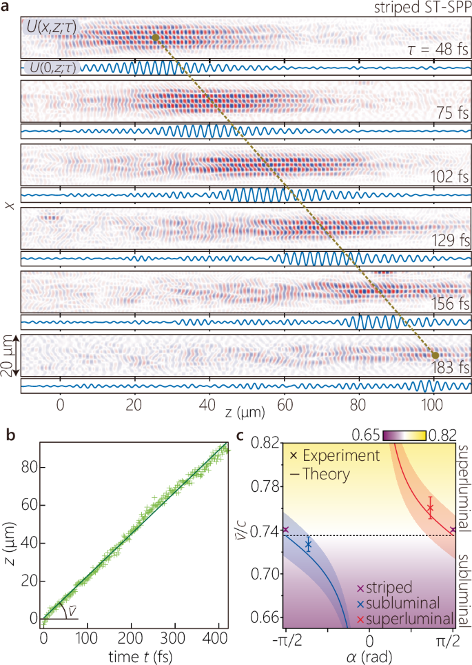
a The real part of the extracted field profiles U(x, z; τ) for a striped ST-SPP at different delays τ (listed on the right). We plot underneath each profile the longitudinal section U(x = 0, z; τ). Each peak position was obtained by least-square fitting with a sinusoidally modulated Gaussian wave packet. b The axial center coordinate z of the peak of the intensity beat-profile from a plotted as a function of real time t (of the propagating striped ST-SPP) calculated from the external delay time τ (of the reference pulse; Methods). The corresponding range of the values of the delay is τ = 0 − 200 fs. c Measured and calculated group velocities for the ST-SPPs (striped, superluminal, and subluminal). The solid curves are the calculated group velocities for ST-SPPs with Δx = 5 μm. The uncertainty bands surrounding the theoretical curves \(\widetilde{v}\) result from a ± 2.5-nm uncertainty in the thickness of the 30-nm-thick fluorescent PMMA layer.
We repeated the procedure for the subluminal and superluminal ST-SPPs, and the estimated group velocities are \({\widetilde{v}}_{-}=(2.18\pm 0.02)\times 1{0}^{8}\) m/s (≈0.73c) and \({\widetilde{v}}_{+}=(2.28\pm 0.03)\times 1{0}^{8}\) m/s (≈0.76c), respectively. The relative relationships of the measured group velocities \({\widetilde{v}}_{-} < {\widetilde{v}}_{{{\rm{SPP}}}} < {\widetilde{v}}_{+}\) are thus consistent with theoretical expectations and with the wavefront tilts in the two-photon fluorescence beat patterns in Fig. 4. We plot in Fig. 6c the measured group velocities compared to \(\widetilde{v}\) calculated as a function of the opening angle α after taking into consideration the uncertainty resulting from the finite accuracy of determining the thickness (30 ± 2.5 nm) of the fluoresecent PMMA layer.