
Dataset description
This paper used the “UCTH Breast Cancer Dataset” for machine learning analysis. The patient data was uploaded to a reliable repository called Mendeley Data in the year 202317. It was obtained from the University of Calabar Teaching Hospital, Nigeria, by observing 213 patients over two years. It contained nine features: age, menopause, tumor size, involved nodes, area of breast affected, metastasis, quadrant affected, previous history of cancer, and diagnosis result. Age and tumor size are continuous variables. Menopause, involved nodes, breast, metastasis, breast quadrant, and history are categorical variables. The categorical target variable is ‘diagnosis result’, which contains ‘0’ for benign and ‘1’ for malignant diagnosis. Table 2 presents a comprehensive description of the features within the dataset.
Table 2 Explanation of the dataset’s features.Statistical preprocessing
The research utilized Jamovi to draw statistical and descriptive conclusions18. The descriptive analysis for continuous variables is given in Table 3. For visualizing the distribution of numerical data, violin plots are shown in Fig. 2. According to the plot, older women are more prone to malignant breast tumors than younger women. Greater tumor size indicated a malignant diagnosis. T-tests were utilized to check the importance of the continuous features. The feature is considered significant if the p-value is less than 0.001. From Table 4 it is concluded that both tumor size and age are necessary features.
Table 3 Descriptive analysis of continuous variables.Fig. 2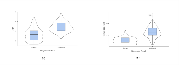
Violin plots. (a) Age (b) Tumor size.
Table 4 Independent samples t-test.
Categorical variables are analyzed using bar plots shown in Fig. 3. It showed the number of patients with benign and malignant tumors for different features. From the graphs, it is interpreted that breast cancer is not adverse in patients who haven’t reached menopause. The diagnosis of this cancer is also observed when the tumor has spread to the auxiliary nodes. Metastasis is noted to be prominent in the case of breast cancer. Malignant tumours have been reported when it affected the upper outer quadrant. Patients with a previous history of cancer are more prone to be diagnosed with this carcinoma. These bar plots help analyze the dataset in-depth. A chi-square test is done to identify significant categorical features. The results are shown in Table 5. The features: Menopause, Involved nodes, Breast Quadrant, and Metastasis are inferred to be necessary attributes as per chi-square tests.
Fig. 3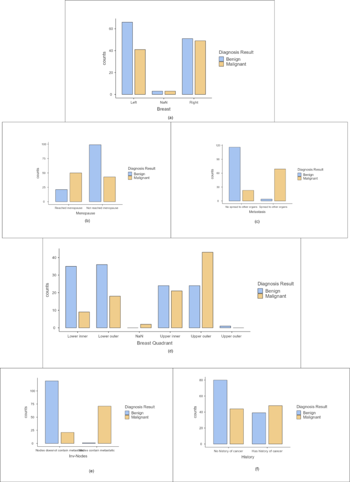
Bar plots for categorical variables (a) Breast (b) Menopause (c) Metastasis (d) Breast quadrant (e) Involved nodes (f) History.
Data preprocessing
Data preprocessing enables converting unprocessed data into a format that is easy to read and use for analysis. This research used preprocessing to avoid using missing values as well as outliers and to optimize the input feature size during analysis. Data shuffling was first done to prevent the model from recalling the order. The dataset had 13 null values, represented as ‘NaN’, that are later removed to attain uniformity. Label encoding was used to convert categorical text data into numerical values since machine learning algorithms need numerical input. It assigns a distinct integer to each category that machine learning algorithms can process. Data scaling avoids any bias towards the larger values in the dataset. Max-Abs-scaling was used to transform all the numbers between 1 and − 1 using its maximum absolute value.
Mutual information and Pearson’s correlation are utilized to determine the important features. The correlation coefficients between any two sets of characteristics are displayed as a heatmap in Pearson’s correlation matrix. The values 1,0 and − 1 indicate positive, zero, and negative correlation, respectively. The heatmap is shown in Fig. 4, according to which Involved nodes, Metastasis, Tumor size, and Age were highly correlated to the diagnosis result. Mutual Information is a univariate filtering method where the significance of a feature is calculated separately. It shows the dependency between two variables with the concept of entropy. In Fig. 5, the qualities are ordered in order of importance. The important features, according to mutual information, are involved nodes, tumor size, metastasis, age, menopause, breast quadrant, and history. The visualization for the distribution of the target variable (diagnostic result) is shown as a pie chart in Fig. 6. From the figure, it is seen that there is a slight imbalance in the data, which might induce biases in the model performance. The Borderline-SMOTE is applied to the training data to balance the classes by creating synthetic samples. This balanced the dataset to 50% for both cases19. Furthermore, the dataset was divided into test and training data in the proportion of 30:70.
Fig. 4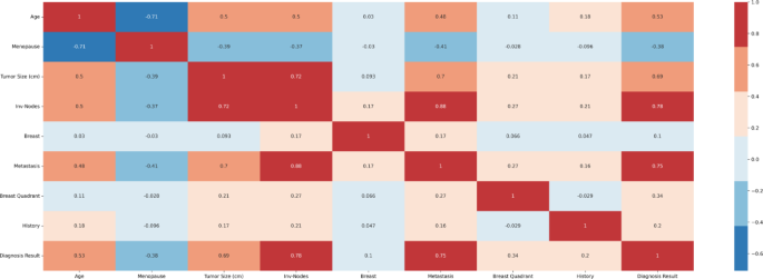
Pearsons correlation heatmap.
Fig. 5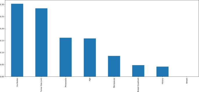
Mutual information of features.
Fig. 6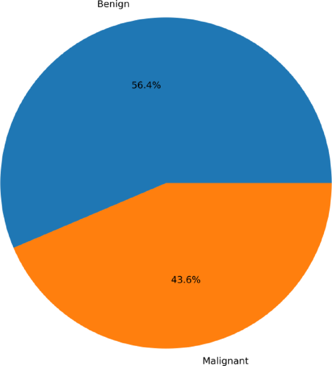 Machine learning and explainable artificial intelligence
The study employed multiple machine learning classification techniques and used a stacking algorithm to combine these classifiers. Eight classifiers used are XGBoost, LightGBM, CatBoost, AdaBoost, KNN, Decision Tree, Logistic Regression, and Random Forest. Although they use different approaches, XGBoost, LightGBM, CatBoost, AdaBoost, and Random Forest integrate multiple tree models for better performance. Decision trees, logistic regression, and K-NN work without combining multiple models. LightGBM and Xgboost are optimal for speed and performance. The outputs from the above classifiers are trained on a meta-classifier by the stacking algorithm. As the stacking methodology integrates the unique strengths from each base model, which improves the model performance by reducing the over-fitting. It also enhances the generalization as it is trained on predictions from the base models, which mitigate biases and errors that are prominent in any single model. The architecture for it is shown in Fig. 7. Hyperparameters are set before training to control how the model learns. It is performed to determine the ideal set of hyperparameters that optimize the model’s performance, generalizing the learning process to respond well to unseen data. GridSearchCV is used for hyperparameter tuning using 5-fold cross-validation in this research. A detailed flowchart of the methodology followed is shown in Fig. 8.
Fig. 7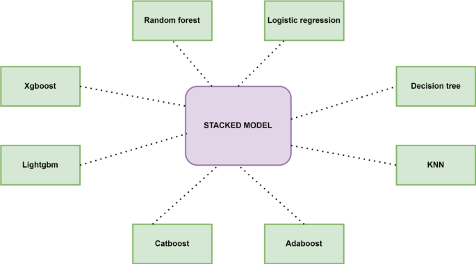
XAI techniques improve the model performance, interpret the results, and provide transparency to the model’s predictions. The necessity for XAI: improve the model’s reliability by identifying the cause for misclassifications; provide transparency to the model, which helps doctors in decision making and for patients to understand the rationale behind the treatment. It also helps identify the important features for the detection of breast cancer. This study used five XAI techniques: SHAP, LIME, Eli5, QLattice, and Anchor. SHAP (Shapley Additive exPlanations) is a method for interpreting complex machine learning models that assigns an important value to each feature known as the Shapley value. These values measure the impact of each input attribute on the model’s predictions20. It provides detailed, individualized explanations for both doctors and patients. The individual feature contribution is critical in refining the model by pinpointing unexpected feature interactions. SHAP is a model-agnostic that can be applied to any machine learning model, in this case, on STACK, a combination of various models. LIME (Local Interpretable Model-agnostic Explanations) is an agnostic model that explains the sample’s local surroundings21. It modifies minor aspects of data to observe the impact of the changes on the predictions, therefore facilitating the identification of the most relevant features. It is especially useful for scenarios involving specific patient predictions. It provides transparency at the individual level. LIME provides flexibility across different models without modification like SHAP. LIME provides explanations that are easy for patients or non-technical stakeholders to understand. Eli5(Explain Like I’m Five) allows us to explain the weights and predictions of the classifiers. It offers global and local explanations22. By analyzing the contributions of different features to the model’s predictions, Eli5 can help identify biases that might have been inadvertently introduced during the model training process. It helps understand the model’s inner workings and troubleshoot the existing issues. For instance, if a model disproportionately weighs a non-relevant feature, it might indicate overfitting or data quality issues. It is a user-friendly interface and an excellent choice for text data, like in this study, as it can explain how input text elements affect the model’s predictions, offering insights into the workings of complex models. QLattice explainability is a technique that looks for patterns and connections in data23. It investigates a broad range of alternative models that offer understandable explanations for the relationships in the data rather than merely fitting the data to a predetermined model. The QLattice model is a set of mathematical expressions that can connect output and input via infinite spatial paths23. Unlike many machine learning models, QLattice focuses on finding simple, interpretable formulas for users to understand how inputs are transformed into outputs, making the models inherently transparent. It identifies key features and provides information on how they interact with each other to affect the outcome. It is robust to new data, as it can adapt by exploring new models, making it responsive to changes in data patterns. Anchor is also a model-agnostic interpretation created by Marco Tulio Ribeiro. It makes use of if-then rules known as anchors24. In medical diagnosis, an anchor might specify that if certain symptoms and test results are present, the diagnosis will invariably be a specific condition. It explains a certain decision by identifying the critical factors that significantly impact it. It accurately describes why a particular decision was made, even if the overall model behavior is complex and non-linear, making it locally faithful. This method helps the user develop confidence in the model by outlining the justification for each prediction. The summary of characteristics of the XAI techniques used is shown in Table 6. Various techniques enhance the reliability and versatility of interpretative outputs through cross-verification of explanations. The study’s XAI techniques complement each other in terms of speed, adaptability, and ease of interpretability for doctors and patients. Due to the different insights in the model’s decision-making process, integrating all five techniques leverages unique strengths.
Table 6 Characteristics of five XAI techniques used.Fig. 8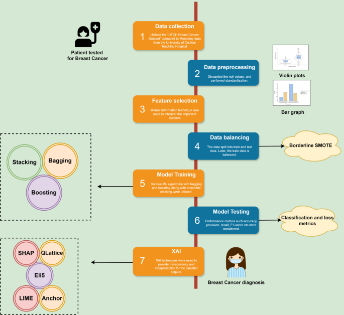
Flow diagram-based methodology.