
Device and setup
Our photon-pressure device, discussed in Fig. 1 and Supplementary Notes 2 and 3, comprises a low-frequency LC circuit with a sweetspot resonance frequency Ω0 = 2π × 446.7 MHz and a high-frequency quantum interference circuit with a sweetspot resonance frequency ω0 = 2π × 8.497 GHz. Both circuits are composed of linear capacitors and multiple linear inductors (cf. Supplementary Note 2) and share as nonlinear inductance and central coupling element a rectangular SQUID. The Josephson elements in the SQUID are monolithic 3D nano-constriction junctions, fabricated by focused neon-ion-beam milling46,47. For maximized photon-pressure coupling rates, the SQUID is galvanically shared by the two circuits, and the LF zero-point-fluctuation currents induce a zero-point-fluctuation flux Φzpf ≈ 198.3 μΦ0 in the SQUID loop (containing both magnetic and kinetic contributions) with the flux quantum Φ0 ≈ 2.068 × 10⁻¹⁵ T m2, cf. Supplementary Note 3. Each of the two circuits is capacitively coupled to an individual coplanar waveguide (CPW) feedline with characteristic impedance Z0 ≈ 50 Ω for driving and readout. Due to the galvanic coupling, the circuits can also be considered a single circuit with a LF and a HF mode, and we will use the words circuit and mode interchangeably in this manuscript.
Fig. 1: Niobium photon-pressure circuits based on a monolithic nano-constriction SQUID and operated in liquid helium.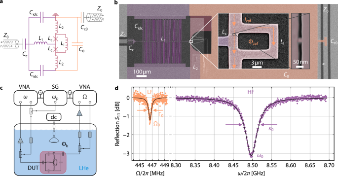
a Simplified circuit equivalent. The HF mode (left half, purple and pink) combines two interdigitated capacitors Cidc with the inductors L1, L2 and Lc. The LF mode (right half, orange and pink) comprises a parallel-plate capacitor C0 with an inductance composed of L2, Ll and Lc. Both modes share the SQUID and parts of the linear inductance (in pink), and each mode is coupled to an individual feedline by coupling capacitors Cc and Cc0, respectively. b False-color scanning electron microscopy image of the device. Colored and light gray parts are Nb, dark gray and transparent parts are Si substrate and Si3N4 dielectric of the LF capacitor, respectively. Color-code equivalent to a. White box inset shows a magnification of the interaction part. The rectangle is the SQUID loop, and the LF zero-point-fluctuation current Izpf flows through the SQUID from top to bottom, hereby threading the loop with a zero-point-fluctuation flux Φzpf. Black box inset shows one of the monolithic 3D nano-constrictions with inductance Lc (image rotated by 90∘). c Simplified experimental setup. The device under test (DUT) is immersed in liquid helium (LHe) and connected to two coaxial lines for readout of the individual modes by a vector network analyzer (VNA). A HF sideband-pump field with frequency ωp from a signal generator (SG) is combined with the HF VNA signal in a directional coupler. Input and output of each readout line are combined by means of further directional couplers and the HF return signal is amplified by a cryogenic amplifier depicted as triangle; the LF mode return signal is amplified by a room-temperature amplifier. A small magnetic-field coil is driven with a direct current (dc) source to induce a bias flux Φb into the SQUID. Gray rectangles represent attenuators. For more details cf. Supplementary Note 1. d Reflection S11 from both circuits (Φb = 0) measured through their individual feedlines. Colored symbols are experimental data, black lines are fit curves. From the fits, we extract the resonance frequencies ω0 = 2π × 8.497 GHz and Ω0 = 2π × 446.7 MHz, as well as the total decay rates κ0 = 2π × 44.9 MHz and Γ0 = 2π × 525 kHz.
As superconducting material for all the metallic parts we chose dc-magnetron sputtered niobium with a critical temperature Tc ≈ 9 K, and as substrate we use high-resistivity intrinsic silicon with a substrate thickness tSi = 525 μm. The bottom niobium layer – defining the HF circuit, the HF CPW feedline center conductor, the SQUID and the bottom electrode of the LF circuit capacitance – has a thickness tNb1 = 120 nm and the top layer – defining the top electrode of the LF capacitance, the LF CPW feedline center conductor, and all ground planes – has tNb2 = 300 nm. As dielectric for the LF parallel-plate capacitors C0 and Cc0 we deposited 200 nm of silicon-nitride by means of plasma-enhanced chemical vapour deposition. All layers have been patterned by maskless optical lithography and reactive-ion-etching (bottom Nb layer) or liftoff (Si3N4 and top Nb layer). Further details regarding device fabrication can be found in “Methods—Device fabrication”.
For the experiments, the 10 × 10 mm2-large chip is wire-bonded to a microwave printed circuit board (PCB) and enclosed in a radiation-tight copper housing. A small electromagnetic coil is mechanically attached to the copper housing in order to apply a dc magnetic field perpendicular to the chip surface and to flux-bias the SQUID. For microwave control and response measurements, both on-chip feedlines are connected via CPWs on the PCB and PCB-SMP connectors to two individual coaxial cables, which combine both input and output (I/O) for each of the circuits by means of a directional coupler. The HF coaxial input line is highly attenuated to equilibrate the feedline thermal noise to the experiment temperature Ts = 4.2 K, and the HF output line is equipped with a cryogenic high-electron-mobility transistor (HEMT) amplifier to maximize the signal-to-noise ratio. On the LF side, both input and output line are slightly attenuated and the returning signal is amplified by a room-temperature HEMT. The two I/O line pairs are connected to individual vector network analyzers (VNAs), and the HF input line is additionally connected to a microwave signal generator, which provides the sideband-pump tone. All experiments reported here were conducted with the sample directly immersed in liquid helium.
As first experiment, we characterize the reflection scattering matrix element S11 of the two circuits via their individual feedlines around their respective resonance frequencies. From fits to the absorption dips, cf. Fig. 1d and “Methods—Resonance fitting”, we extract the resonance frequencies of both modes (given above) as well as their internal and external decay rates κint = 2π × 38.2 MHz, κext = 2π × 6.7 MHz for the HF circuit and Γint = 2π × 489 kHz, Γext = 2π × 36 kHz for the LF circuit; data were taken at the flux sweetspot. Both circuits are undercoupled with κint/κext > 1 and Γint/Γext > 1. The high value for κint can be attributed to the nano-constrictions, which have been shown to have a suppressed critical temperature and therefore considerable quasiparticle losses at 4.2 K46,47. However, this is not detrimental for the current experiment, but rather desired, since the high κint is directly related to the dissipative coupling contribution. The large Γint/Γext has the advantage that the LF circuit does not need much attenuation in addition to the cable-attenuation to reach an effective mode temperature TLF ≲ 10 K, which is a big advantage if a cryogenic LF amplifier is not available (as was the case for our experiment).
Flux-tunable photon-pressure interactions
The dispersive and dissipative single-photon coupling rates of a photon-pressure system are given by
$${g}_{0\omega }=-\frac{\partial {\omega }_{0}}{\partial {\Phi }_{{\rm{b}}}}{\Phi }_{{\rm{zpf}}}$$
(1)
$${g}_{0\kappa }=-\frac{\partial {\kappa }_{0}}{\partial {\Phi }_{{\rm{b}}}}{\Phi }_{{\rm{zpf}}},$$
(2)
respectively, with the bias flux though the SQUID Φb. Hence, to characterize the system and to select a good working point for the further experiments, as a next step we investigate the response of the HF resonance frequency and linewidth with respect to applied flux Φb. We sweep the current through the attached coil, and for each current value we take a trace of both the HF and the LF reflection with the VNAs. Although the LF circuit is also weakly flux dependent (cf. Supplementary Note 3), we focus our discussion on the HF mode here, since its properties determine the interaction between the circuits. Our findings are summarized in Fig. 2.
Fig. 2: Dispersive and dissipative photon-pressure coupling rates and their tuning with bias flux through the SQUID.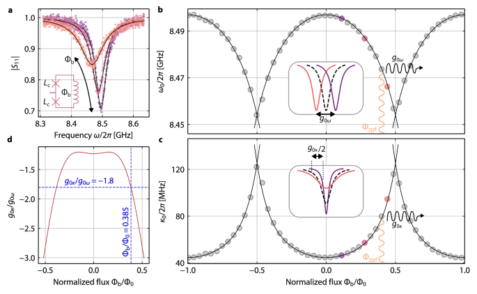
a Reflection ∣S11∣ of the HF mode for three different bias-flux values 0.1 ≲ Φb/Φ0 ≲ 0.45. With increasing bias flux, the resonance frequency shifts to lower values and the total linewidth increases. Symbols are data, lines are fits. The frequency-shift can be understood as an increase of the nonlinear constriction inductance Lc with increasing flux through the SQUID loop (cf. inset), the increase in linewidth by current-induced quasiparticles. b Resonance frequencies ω0(Φb), extracted from fits to reflection data S11 (cf. a), which show a periodic modulation with period Φ0. Circles are data, line is a fit (cf. Supplementary Note 3). If the SQUID is biased to a constant value Φb/Φ0 ≈ 0.385 and additional oscillating zero-point-fluctuation flux from the LF mode Φzpf ≈ 198.3 μΦ0 threads the SQUID, this leads to a modulation of the HF resonance frequency. The total frequency-modulation induced by Φzpf is equivalent to the dispersive single-photon coupling rate g0ω = 2π × 27.1 kHz. Inset schematic visualizes g0ω. c Analogous to panel b, but for the total HF linewidth κ0, which periodically modulates between ~ 44.5 MHz and ~ 125 MHz, revealing that despite the large decay rates the device is in the sideband-resolved limit with Ω0/κ0 ≳ 3.5 for all Φb. Circles are data, line is a polynomial fit (cf. Supplementary Note 3). At the operation point Φb/Φ0 = 0.385, the LF flux Φzpf induces a dissipative photon-pressure interaction with single-photon coupling rate g0κ = − 2π × 48.8 kHz. Inset schematic visualizes g0κ. d Ratio of dissipative to dispersive single-photon coupling rate g0κ/g0ω vs. Φb, which is calculated from the fit curves in b and c. At the operation point for this work (marked by the crossing point of the blue dashed lines), we find g0κ/g0ω ≈ − 1.8.
Upon increasing Φb starting at the sweetspot Φb = 0, we observe a redshift of the HF resonance frequency and an increase of the linewidth. Over a larger flux range, we observe that both quantities periodically modulate with period Φ0 as expected for a SQUID due to fluxoid quantization. Note however, that ω0 and κ0 = κint + κext modulate with opposite trend, i.e., when ω0 decreases κ0 increases and vice versa. The maximum resonance frequency is found at the sweetspots Φb/Φ0 = n with \(n\in {\mathbb{Z}}\), while this is the flux of the lowest decay rate. The modulation range for the resonance frequency is \({\omega }_{0}^{\max }-{\omega }_{0}^{\min }\approx 2\pi \times 43\,{\mathrm{MHz}}\) and for the linewidth \({\kappa }_{0}^{\max }-{\kappa }_{0}^{\min }\approx 2\pi \times 81\,{\mathrm{MHz}}\), i.e., κ0 changes by about twice the amount ω0 does. From fits to the data points (for details see Supplementary Note 3), we determine the derivatives for both parameters to calculate the single-photon coupling rates g0ω and g0κ. Additionally, we obtain the ratio of the derivatives as a function of Φb, which is equal to the flux-dependent ratio of the coupling rates g0κ/g0ω.
As a good compromise between low circuit nonlinearity, medium total decay rate and maximum slope of both the tuning arcs, we choose the operation point Φb/Φ0 ≈ 0.385. Combining all parameters, we determine the dispersive and dissipative single-photon coupling rates at this flux point as g0ω = 2π × 27.1 kHz and g0κ = 2π × − 48.8 kHz, respectively, which correspond to a large ratio g0κ/g0ω ≈ − 1.8. Note that depending on the exact flux-bias point, this ratio can be tuned between − 1.2 and − 3, cf. Fig. 2d. The HF resonance frequency and linewidth at the working point are ω0 ≈ 2π × 8.476 GHz and κ0 ≈ 2π × 73.9 MHz; the LF parameters are Ω0 ≈ 2π × 446.3 MHz and Γ0 ≈ 2π × 601 kHz. The external decay rates are nearly constant as a function of flux, and so all the variation of κ0 with Φb and Φzpf can be attributed to κint, cf. Supplementary Note 3. Note though, that in general it is important to discriminate between internal and external dissipative photon-pressure, since they can lead to qualitatively and quantitatively different consequences; here \({g}_{0{\kappa }_{\mathrm{int}}}={g}_{0\kappa }\) and \({g}_{0{\kappa }_{\mathrm{ext}}}\approx 0\). Combined with the self-Kerr nonlinearity of the HF mode \({{\mathcal{K}}}\approx 2\pi \times -5.4\,{\mathrm{kHz}}\) (the LF self-Kerr is negligibly small), cf. Supplementary Note 7, the device is well in the sideband-resolved regime with Ω0/κ0 ≈ 6 while in principle allowing for strong sideband pump tones due to \({{\mathcal{K}}}/{\kappa }_{0}\ll 1\).
Photon-pressure induced Fano-transparency
To experimentally investigate the effects of the dissipative coupling contribution to the overall dynamics of the circuits, we begin with the protocol of photon-pressure induced transparency (PPIT). Here, a strong, fixed-frequency sideband-pump field is sent to the HF cavity around its red sideband \({\omega }_{\mathrm{p}}={\omega }_{0}^{{\prime} }-{\Omega }_{{\mathrm{eff}}}+{\delta }_{{\mathrm{eff}}}\) with \(| {\delta }_{{\mathrm{eff}}}| \le {\kappa }_{0}^{{\prime} }/4\), and a much weaker VNA probe tone with frequency \(\omega \sim {\omega }_{0}^{{\prime} }\) is used to characterize the modified HF reflection response in a frequency span of few \({\kappa }_{0}^{{\prime} }\) around \({\omega }_{0}^{{\prime} }\), cf. Fig. 3a. We prime all HF mode quantities here to indicate that they shift with the intracavity pump photon number nc due to the Kerr nonlinearity and a nonlinear damping. The effective LF mode frequency \({\Omega }_{\mathrm{eff}}={\Omega }_{0}^{{\prime} }+\delta {\Omega }_{\mathrm{pp}}\) contains both, the power-shifted LF frequency due to a potential cross-Kerr effect \({\Omega }_{0}^{{\prime} }\) and possible dynamical backaction contributions δΩpp, which we do not know at this point and therefore choose Ωeff as reference for the cavity red sideband. However, for all our data Ωeff − Ω0 < Γ0, hence the difference is very small.
Fig. 3: Fano-transparency indicates interference of dispersive and dissipative photon-pressure.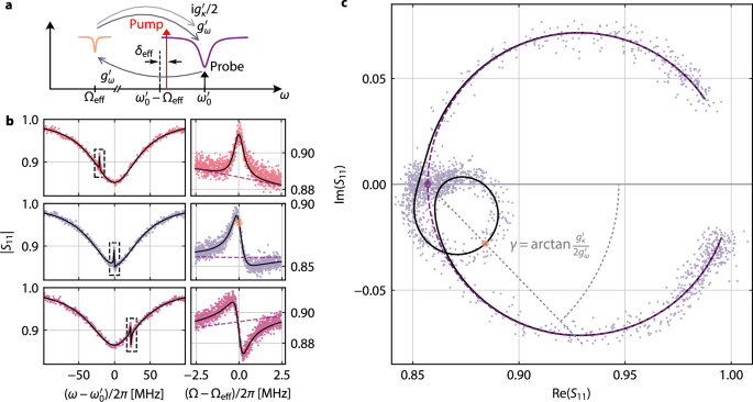
a Schematic of the experimental setting for the observation of photon-pressure induced transparency (PPIT). A strong microwave pump tone (red vertical arrow) with power Pp and frequency \({\omega }_{\mathrm{p}}={\omega }_{0}^{{\prime} }-{\Omega }_{{\mathrm{eff}}}+{\delta }_{{\mathrm{eff}}}\) is sent to the device around the red sideband of the HF cavity. A small VNA probe tone (black vertical arrow) with relative frequency Ω = ω − ωp scans the HF reflection around \({\omega }_{0}^{{\prime} }\). The beating of the pump and probe tones coherently drives the LF mode with a strength proportional to the dispersive coupling rate \({g}_{\omega }^{{\prime} }\). The resulting LF amplitude in turn induces both a dispersively and a dissipatively generated sideband to the pump tone at ωp + Ω, which are \(\propto \,{g}_{\omega }^{{\prime} }\) and \(\propto \, {\mathrm{i}}{g}_{\kappa }^{{\prime} }/2\), respectively, and which both interfere with the original probe tone. b HF cavity reflection ∣S11∣ in the presence of a pump tone for three different pump detunings \({\delta }_{{\mathrm{eff}}}={( – {\kappa }_{0}^{{\prime} }/4, 0 ,+ {\kappa }_{0}^{{\prime} }/4)}\) (from top to bottom). Data in left graphs are vs. detuning from HF cavity resonance \(\omega -{\omega }_{0}^{{\prime} }\), and clear PPIT signatures can be identified when \(\omega -{\omega }_{0}^{{\prime} }\approx {\delta }_{{\mathrm{eff}}}\). The smaller graphs on the right show zooms to the transparency resonances (dashed boxes in left graphs) plotted vs. detuning from ωp + Ωeff. Symbols are data, lines are fits. The point of PPIT resonance in the zoom for δeff ≈ 0 is marked with an orange disk, and the cavity reflection for \({g}_{\omega }^{{\prime} }={g}_{\kappa }^{{\prime} }=0\) is added as dashed purple line in all zooms. c The dataset for δeff ≈ 0 in complex representation. Points are data, black line is a theory curve with all parameters from the fit and δeff = 0. The cavity resonance traces a large circle anchored at (1, 0), the PPIT signature traces a smaller circle anchored on the resonance point of the bare cavity (purple disk); the resonance point of the PPIT is marked with the orange disk. For \({g}_{\kappa }^{{\prime} }=0\), the PPIT circle would point towards (1, 0) and the dashed line connecting the two resonance points would be the real axis. However, the presence of dissipative coupling leads to a rotation of the PPIT circle around its anchor point by an angle \(\gamma=\arctan (g_\kappa^{\prime} /2{g}_{\omega }^{{\prime} })\). Here, we obtain γ ≈ − 46 ∘, which corresponds to \({g}_{\kappa }^{{\prime} }/{g}_{\omega }^{{\prime} }\approx -2.1\).
The beating of the pump and probe tones in the PPIT protocol coherently drives the LF circuit into oscillation, which in turn generates a sideband field to the pump tone, that interferes with the original probe tone with a phase-relation determined by the interaction and the detuning. As a consequence, a narrow transparency window with the shape of the effective LF susceptibility appears within the HF cavity resonance, a phenomenon closely related to EIT in atomic systems48 and OMIT in optomechanical devices49. An interesting question is now whether and how the presence of dissipative coupling alters the usual, purely dispersive PPIT signature.
To model and understand the experiment, we derive the linearized equations of motion for the HF cavity field \(\hat{c}\) and the LF mode field \(\hat{d}\), which are given by
$${\dot{\hat{c}}}=\left[-{{\rm{i}}}\Delta ^{\prime}_{{\rm{p}}} -\frac{{\kappa }_{0}^{{\prime} }}{2}\right]\hat{c}-{{\rm{i}}}\left[{g}_{\omega }^{{\prime} }+{{\rm{i}}}\frac{{g}_{\kappa }^{{\prime} }}{2}\right]\left(\hat{d}+{\hat{d}}^{{\dagger} }\right)+{\mathrm{i}}\sqrt{{\kappa_{{\rm{ext}}} ^{\prime}} }{\hat{c}}_{\mathrm{in}}$$
(3)
$$\dot{\hat{d}}=\left[{\mathrm{i}}{\Omega }_{0}^{{\prime} }-\frac{{\Gamma }_{0}^{{\prime} }}{2}\right]\hat{d}-{\mathrm{i}}{g}_{\omega }^{{\prime} }\left(\hat{c}+{\hat{c}}^{{\dagger} }\right)$$
(4)
where \(\Delta^{\prime}_{\mathrm{p}}={\omega}_{\mathrm{p}}-{\omega}_{0}^{{\prime}}\), \({\hat{c}}_{\mathrm{in}}\) represents the input probe tone, and \({g}_{\omega }^{{\prime} }\) and \({g}_{\kappa }^{{\prime} }\) are the dispersive and dissipative multiphoton coupling rates. We omit any input noise here, since it can be neglected to first order in a PPIT experiment, that is only considering the response to a coherent input tone. A complete derivation of the equations of motion can be found in Supplementary Notes 4 and 5.
One very interesting detail in the equations of motion is an asymmetry in the coupling terms. While the HF mode is coupled to the LF mode with a term \(\propto g^{\prime}={g}_{\omega }^{{\prime} }+{\mathrm{i}}{g}_{\kappa }^{{\prime} }/2\), only the dispersive interaction \({g}_{\omega }^{{\prime} }\) contributes explicitly to changes of the LF mode field. In other words, the LF mode is driven proportional to \({g}_{\omega }^{{\prime} }\) only, while the HF sideband is generated via \({g}_{\omega }^{{\prime} }+{\mathrm{i}}{g}_{\kappa }^{{\prime} }/2\). By solving the equations of motion using Fourier transformation, combining the results, and applying the high-Q limit for the LF mode (cf. Supplementary Note 5), we arrive at an expression for the HF reflection, when probed around resonance
$${S}_{11}=1-\kappa_{{\rm{ext}}}^{\prime} {\chi ^{\prime}_{\mathrm{c}}} \left[1-{g}_{\omega }^{{\prime} }\left({g}_{\omega }^{{\prime} }+{\mathrm{i}}\frac{{g}_{\kappa }^{{\prime} }}{2}\right){\chi ^{\prime}_{\mathrm{c}}} {\chi }_{0}^{{\mathrm{eff}}}\right]$$
(5)
with the HF susceptibility \({\chi}^{\prime}_{\mathrm{c}}=[{\kappa }_{0}^{{\prime}}/2+{\mathrm{i}}({\Delta}^{\prime}_{\mathrm{p}}+\Omega )]^{-1}\), the effective LF susceptibility \({\chi }_{0}^{{\mathrm{eff}}}={[{\Gamma }_{0}^{{\prime} }/2+{\mathrm{i}}(\Omega -{\Omega }_{0}^{{\prime} })+\Sigma ]}^{-1}\), the dynamical backaction \(\Sigma={g}_{\omega }^{{\prime} }(g^{\prime} \chi^{\prime}_{{\mathrm{c}}0} -g^{\prime*}\overline{\chi}^{\prime}_{{\mathrm{c}}0})\), \(\chi^{\prime}_{{\mathrm{c}}0}=\chi^{\prime}_{\mathrm{c}} ({\Omega }_{0}^{{\prime} })\), \(\overline{\chi}^{\prime}_{{\mathrm{c}}0}=\chi^{\prime*}_{\mathrm{c}}(-{\Omega }_{0}^{{\prime} })\) and the probe frequency relative to the pump Ω = ω − ωp. Note that without dispersive coupling \({g}_{\omega }^{{\prime} }=0\) there would be no PPIT at all and no dynamical backaction, but both effects are nevertheless considerably modified by the presence of \({g}_{\kappa }^{{\prime} }\) in \(g^{\prime}\). If we had an external-dissipative interaction instead of (or in addition to) the internal-dissipative one, the equations of motion and the reflection expression would contain additional terms and neither the dynamical backaction nor the PPIT signature would vanish for \({g}_{\omega }^{{\prime} }=0\)34.
As a consequence of \({g}_{\kappa }^{{\prime} }\ne 0\), experiment and theory both reveal an interference-based and Fano-like modification of the PPIT resonance within the HF cavity resonance, cf. Fig. 3b. Most striking are two features. First, we have an asymmetric PPIT lineshape when the pump is directly on the effective red sideband \({\delta }_{{\mathrm{eff}}}={\omega }_{\mathrm{p}}-({\omega }_{0}^{{\prime} }-{\Omega }_{{\mathrm{eff}}})\approx 0\) in contrast to dispersive coupling only. And secondly, the usual mirror symmetry for + δeff and − δeff is not preserved anymore. In the complex representation of S11, cf. Fig. 3c, the origin of this additional tilt becomes apparent. Usually (i.e. for \({g}_{\kappa }^{{\prime} }=0\)), the PPIT describes a small circle within the much larger HF cavity resonance circle, but both have their anchor points and their centers on the real axis for the pump on the red sideband. Due to the additional phase shift of π/2 of the dissipative coupling term (i = eiπ/2), however, the PPIT circle gets rotated around its anchor point.
Evaluating Eq. (5) at the corresponding frequency points (cf. “Methods—Fano-angle in transparency experiment” and Supplementary Note 6) reveals that in fact the angle γ between the two circle axes is given by
$$\tan \gamma=\frac{{g}_{\kappa }^{{\prime} }}{2{g}_{\omega }^{{\prime} }}.$$
(6)
For the dataset discussed in Fig. 3, we find γ = − 46∘, which is equivalent to \({g}_{\kappa }^{{\prime} }/{g}_{\omega }^{{\prime} }\approx -2.1\). Observing this tilt is therefore not only a clear confirmation for the presence of internal-dissipative photon-pressure coupling, but also might be a very useful and extraordinarily fast and simple method to quantify internal-dissipative coupling rates in the first place. It only requires a single complex resonance measurement and especially in devices, which do not provide the possibility to tune a system parameter p to extract the derivatives of ∂ω0/∂p and ∂κ0/∂p (e.g. in most optomechanical systems), the transparency rotation angle can be of high relevance. In this context it is also noteworthy, that external-dissipative photon-pressure does not result in the same Fano-interference in the sideband-resolved limit and with a pump tone around one of the sidebands, since its main consequence is a detuning-dependent re-scaling of \({g}_{\omega }^{{\prime} }\) instead of adding an imaginary component to the total coupling rate34.
The value of \({g}_{\kappa }^{{\prime} }/{g}_{\omega }^{{\prime} }\approx -2.1\) we find here from the PPIT data is only close to the single-photon equivalent g0κ/g0ω ≈ − 1.8 obtained in the context of Fig. 2, but not exactly the same. The latter, i.e., \({g}_{0\kappa }/{g}_{0\omega }={g}_{\kappa }^{{\prime} }/{g}_{\omega }^{{\prime} }\), would be expected if the multiphoton coupling rates scaled with pump photon number nc as usual as \({g}_{\omega }^{{\prime} }=\sqrt{{n}_{\mathrm{c}}}{g}_{0\omega }\) and \({g}_{\kappa }^{{\prime} }=\sqrt{{n}_{\mathrm{c}}}{g}_{0\kappa }\). The difference found here is not caused by inaccuracies, however, it rather points towards another highly interesting effect, which will be addressed in the next section.
Nonlinearity-enhanced coupling rates
When performing the PPIT experiment with varying pump power and detuning, we observe that resonance frequencies, linewidths and coupling rates, and surprisingly even \({g}_{\kappa }^{{\prime} }/{g}_{\omega }^{{\prime} }\), depend on pump power. The shift of \({\omega }_{0}^{{\prime} }\) is explained by the Kerr anharmonicity of the HF mode, which stems from the nonlinear superconducting inductances. The origin of the nonlinear linewidth broadening, which is clearly faster than linear in pump photon number, cf. Fig. 4b, are ac-current-induced quasiparticles and an ac-current-induced suppression of the superconducting gap in the constrictions. We observe, consistent with that interpretation, that \(\kappa^{\prime}_{\mathrm{ext}}\) is not significantly modified by the pump. The pump-broadened linewidth is phenomenologically modeled using \({\kappa }_{0}^{{\prime} }={\kappa }_{0}+2{\kappa }_{1}{n}_{\mathrm{c}}+3{\kappa }_{2}{n}_{\mathrm{c}}^{2}+4{\kappa }_{3}{n}_{\mathrm{c}}^{3}\) with κ0 = 2π × 70.7 MHz and the nonlinear-damping coefficients κ1 ≈ 2π × 3.7 kHz, κ2 ≈ 0, and κ3 ≈ 2π × 0.37 mHz; all values are obtained from a fit to the data. For the origin of the prefactors 2, 3 and 4 in the nonlinear contributions, cf. Supplementary Note 4.
Fig. 4: Nonlinear damping and nonlinearity-enhanced photon-pressure coupling.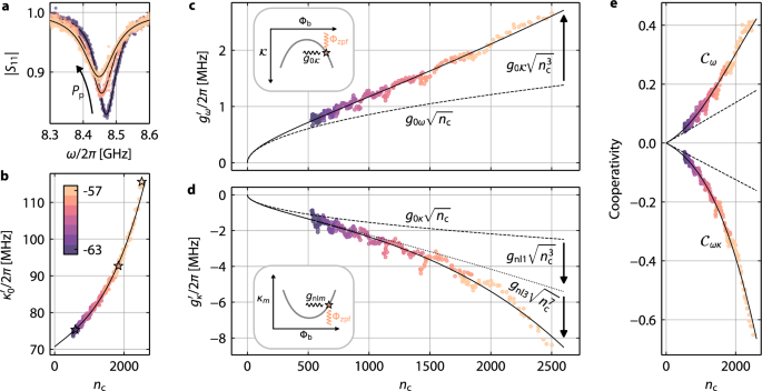
a HF cavity reflection ∣S11∣ for fixed ωp = 2π × 8.031 GHz and increasing sideband pump-power Pp, measured by a small VNA probe tone. With increasing pump power, the cavity shifts to lower frequencies due to its Kerr anharmonicity, and its linewidth increases due to nonlinear damping. Symbols are experimental data, lines are fits. b Total HF mode linewidth \({\kappa }_{0}^{{\prime} }\) for seven different pump powers (color-coded as given by the color bar in units of dBm) and multiple detunings between \(-{\kappa }_{0}^{{\prime} }/4\) and \(+{\kappa }_{0}^{{\prime} }/4\) in pump-frequency steps of 2 MHz, all plotted vs. their corresponding intracavity pump photon-number nc. Symbols are data, star symbols correspond to the datasets in a. Line is a fit with \({\kappa }_{0}^{{\prime} }={\kappa }_{0}+2{\kappa }_{1}{n}_{\mathrm{c}}+ 3{\kappa }_{2}{n}_{\mathrm{c}}^{2}+ 4{\kappa}_{3}{n}_{\mathrm{c}}^{3}\). c Dispersive multiphoton coupling rate \({g}_{\omega }^{{\prime} }\) vs. nc as extracted from PPIT. Pump powers and detunings are identical to b. Symbols are data, solid line is a fit with \({g}_{\omega }^{{\prime} }={g}_{0\omega }\sqrt{{n}_{\mathrm{c}}}+{g}_{0{{\mathcal{K}}}}\sqrt{{n}_{\mathrm{c}}^{3}}\); dashed line shows \({g}_{\omega }={g}_{0\omega }\sqrt{{n}_{\mathrm{c}}}\) without the Kerr enhancement. Inset: Schematic of the HF self-Kerr nonlinearity \({{\mathcal{K}}}\) as a function of bias flux and how the LF zero-point-fluctuation flux modulates it by \({g}_{0{{\mathcal{K}}}}=-{\Phi }_{\mathrm{zpf}}\partial {{\mathcal{K}}}/\partial {\Phi }_{\mathrm{b}}\). d Dissipative multiphoton coupling rate \({g}_{\kappa }^{{\prime} }\) vs. nc as extracted from PPIT. Pump powers and detunings are identical to b. Symbols are data, solid line is a fit with \({g}_{\kappa }^{{\prime} }={g}_{0\kappa }\sqrt{{n}_{\mathrm{c}}}+{g}_{\mathrm{nl}1}\sqrt{{n}_{\mathrm{c}}^{3}}+{g}_{\mathrm{nl}2}\sqrt{{n}_{\mathrm{c}}^{5}}+{g}_{\mathrm{nl}3}\sqrt{{n}_{\mathrm{c}}^{7}}\); dashed line shows \({g}_{\kappa }={g}_{0\kappa }\sqrt{{n}_{\mathrm{c}}}\) without nonlinearity-enhancement, dotted line shows \({g}_{0\kappa }\sqrt{{n}_{\mathrm{c}}}+{g}_{\mathrm{nl}1}\sqrt{{n}_{\mathrm{c}}^{3}}\). From the fit, we obtain gnl2 ≈ 0. Inset: Schematic of a generic nonlinear damping coefficient κm, \(m\in {\mathbb{N}}\), as a function of bias flux and how the LF zero-point-fluctuation flux modulates it by gnlm = − Φzpf∂κm/∂Φb. e Dispersive cooperativity \({{{\mathcal{C}}}}_{\omega }=4{g}_{\omega }^{{\prime} 2}/{\kappa }_{0}^{{\prime} }{\Gamma }_{0}\) and cross-cooperativity \({{{\mathcal{C}}}}_{\omega \kappa }=2{g}_{\omega }^{{\prime} }{g}_{\kappa }^{{\prime} }/{\kappa }_{0}^{{\prime} }{\Gamma }_{0}\) vs. nc. Symbols are derived from data, solid lines follow from the fits in b–d with Γ0 = 2π × 601 kHz, dashed line is the reference without the nonlinearity-enhancement and with constant \({\kappa }_{0}^{{\prime} }={\kappa }_{0}\). The effects from increasing \({\kappa }_{0}^{{\prime} }\) and nonlinearity-enhanced \({g}_{\omega }^{{\prime} },{g}_{\kappa }^{{\prime} }\) compete, but overall still lead to a significant enhancement of both cooperativities by factors up to ~ 2.4 and ~ 4.1, respectively.
Finally, we investigate \({g}_{\omega }^{{\prime} }\) and \({g}_{\kappa }^{{\prime} }\) as a function of pump photon number. A description of how we obtained the values from PPIT data is given in “Methods—Extracting the multiphoton coupling rates”. In Fig. 4, we show all the multiphoton coupling rates obtained for multiple pump powers and detunings vs. nc, and what we observe is surprising and exciting. Both coupling rates do not scale \(\propto \sqrt{{n}_{\mathrm{c}}}\) as expected from a simple first-order theory, but they increase considerably faster. While \({g}_{\omega }^{{\prime} }\) seems to grow almost linearly, but with a finite value at nc = 0, \({g}_{\kappa }^{{\prime} }\) grows even faster, in particular at the highest photon numbers, similar to the increase of \({\kappa }_{0}^{{\prime} }\) with nc. For the lowest pump powers, the ratio \({g}_{\kappa }^{{\prime} }/{g}_{\omega }^{\prime}\) is very close to g0κ/g0ω = − 1.8, for the highest photon numbers though \({g}_{\kappa }^{{\prime} }/{g}_{\omega }^{{\prime} }\to -3.1\). The PPIT data in Fig. 3 are in the intermediate \({g}_{\kappa }^{{\prime} }/{g}_{\omega }^{{\prime} }\)-regime (taken at Pp = − 58 dBm, i.e., nc ≈ 1570 for δeff ≈ 0), which explains the discrepancy between g0κ/g0ω = − 1.8 and \({g}_{\kappa }^{{\prime} }/{g}_{\omega }^{{\prime} }=-2.1\) found from γ.
Nonlinearity-enhanced multiphoton coupling rates are an intriguing and potentially very useful observation, which can be explained as follows. Each of the nonlinearity parameters \({{\mathcal{K}}}\), κ1, κ2 and κ3 is flux-dependent46, i.e., modulated by Φzpf, and hence each can be the origin of an additional type of photon-pressure coupling. To first order, these additional coupling rates on the single-photon level are
$${g}_{0{{\mathcal{K}}}}=-\frac{\partial {{\mathcal{K}}}}{\partial {\Phi }_{{\rm{b}}}}{\Phi }_{{\rm{zpf}}},\,{g}_{{\rm{nl}}m}=-\frac{\partial {\kappa }_{m}}{\partial {\Phi }_{{\rm{b}}}}{\Phi }_{{\rm{zpf}}},\,m\in {\mathbb{N}}$$
(7)
and intrinsically they are several orders of magnitude smaller than g0ω and g0κ. In the framework of the linearized equations of motion, however, they get integrated into the multiphoton coupling rates as
$${g}_{\omega }^{{\prime} }={g}_{0\omega }\sqrt{{n}_{\mathrm{c}}}+{g}_{0{{\mathcal{K}}}}\sqrt{{n}_{\mathrm{c}}^{3}}$$
(8)
$${g}_{\kappa }^{{\prime} }={g}_{0\kappa }\sqrt{{n}_{{\rm{c}}}}+{g}_{{\rm{nl1}}}\sqrt{{n}_{\mathrm{c}}^{3}}+{g}_{\mathrm{nl}2}\sqrt{{n}_{\mathrm{c}}^{5}}+{g}_{\mathrm{nl}3}\sqrt{{n}_{\mathrm{c}}^{7}},$$
(9)
which means that despite their smallness on the single-photon level they can be very significant in the high-pump-power regime. Interestingly, also here we find a vanishing second order gnl2 ≈ 0 from a corresponding fit, and for the finite coupling rates we get \({g}_{0{{\mathcal{K}}}} \approx 2\pi \times 10.0\,{\mathrm{Hz}}\), gnl1 ≈ 2π × − 22.1 Hz and gnl3 ≈ 2π × − 3.5 μHz. Table 1 summarizes all the relevant nonlinearity coefficients for \({\omega }_{0}^{{\prime} }\), \({\kappa }_{0}^{{\prime} },{g}_{\omega }^{{\prime} }\) and \({g}_{\kappa }^{{\prime} }\).
Table 1 Nonlinearity coefficients for \({\omega }_{0}^{{\prime} },{\kappa }_{0}^{{\prime} },{g}_{\omega }^{{\prime} }\) and \({g}_{\kappa }^{{\prime} }\)
For the Kerr constant, this effect has been predicted by theoretical work50,51, and a related observation of much smaller magnitude has been reported in a multi-tone driven photon-pressure experiment20. The dissipative case, however, is even more impactful in our work than the dispersive one. While \({g}_{\omega }^{{\prime} }\) is roughly doubled in the high-power regime compared to \({g}_{0\omega }\sqrt{{n}_{\mathrm{c}}}\), which is already impressive, the dissipative multiphoton coupling \({g}_{\kappa }^{{\prime} }\) gets boosted by up to a factor ~ 3.4 compared to \({g}_{\kappa }={g}_{\kappa 0}\sqrt{{n}_{\mathrm{c}}}\), cf. Fig. 4. Often, it is insightful to consider the cooperativity instead of the coupling rates, especially, when also the mode linewidth is a function of nc as is the case here. Unfortunately, the purely dissipative cooperativity \({{{\mathcal{C}}}}_{\kappa }={g}_{\kappa }^{{\prime} 2}/{\kappa }_{0}^{{\prime} }{\Gamma }_{0}\) plays no role in this experiment due to the nonreciprocity of the interaction, but it would be enhanced by almost one order of magnitude. The dispersive cooperativity \({{{\mathcal{C}}}}_{\omega }=4{g}_{\omega }^{{\prime} 2}/{\kappa }_{0}^{{\prime} }{\Gamma }_{0}\) and the cross-cooperativity \({{{\mathcal{C}}}}_{\omega \kappa }=2{g}_{\omega }^{{\prime} }{g}_{\kappa }^{{\prime} }/{\kappa }_{0}^{{\prime} }{\Gamma }_{0}\), on the other hand, are important for e.g. dynamical backaction (see below) and perspectively for sideband-cooling or parametric amplification. Those two cooperativities are still enhanced by a factor ~ 2.4 and ~ 4.1, respectively, which shows that the enhancement of the coupling rates by far overcompensates the increase of \({\kappa }_{0}^{{\prime} }\).
Potentially, such cooperativity enhancements could lead to low-power groundstate-cooling or increased flux/displacement sensitivity, with a particular usefulness in optomechanics, where single-photon coupling rates are often very small compared to photon-pressure circuits and where device or setup heating by large pump powers is sometimes a limiting factor. Especially in superconducting circuits, it is furthermore possible to design \({{\mathcal{K}}}\) and correspondingly \(\partial {{\mathcal{K}}}/\partial {\Phi }_{{\rm{b}}}\) by carefully considered junction arrays52, which might facilitate \({g}_{0{{\mathcal{K}}}}\) to be increased further by orders of magnitude in future systems.
The data in Fig. 4c and d also confirm once more, that the external-dissipative coupling rate plays no role here. If a significant contribution from \({g}_{{\kappa }_{\mathrm{ext}}}\) was present in the device, this would lead to a dependence of the effective \({g}_{\omega }^{{\prime} }\) on the detuning between pump and HF resonance \(\Delta^{\prime}_{\mathrm{p}}\)34, which would have two notable consequences. First, not all the data for \({g}_{\omega }^{{\prime} }\) in c would fall onto a single line, but within each color the values for high photon numbers would be pushed down (up), if \({g}_{0{\kappa }_{\mathrm{ext}}} < 0\) (\({g}_{0{\kappa }_{\mathrm{ext}}} > 0\)), and the values for low photon numbers would be pushed up (down). And secondly, the ratio \({g}_{\kappa }^{{\prime} }/{g}_{\omega }^{{\prime} }\) would deviate considerably from the flux arc-based values even for very small nc, cf. also Supplementary Note 6. Even though some scattering of both coupling rates is visible, none of the two effects is observed within the experimental accuracy.
Dynamical backaction
Finally, we analyze the dynamical backaction exerted from the HF intracavity fields to the LF circuit as a function of power and detuning. This is not only an essential quantity for future experiments and applications like sideband-cooling with dissipative interactions, but an agreement with theoretical predictions will also serve as independent confirmation of our above conclusions, including the existence and strength of the dissipative coupling, the nonlinear enhancement of \({{{\mathcal{C}}}}_{\omega }\) and \({{{\mathcal{C}}}}_{\omega \kappa }\), and the photon-number dependent ratio of \({g}_{\omega }^{{\prime} }/{g}_{\kappa }^{{\prime} }\). Dynamical backaction arises from the time-delayed adjustments of the pump fields in the HF mode to changes of ω017,53, here in our system caused by a change of flux through the SQUID. Hence, it depends on detuning between pump and cavity and on the cavity decay rate, which determines the time scale, on which this adjustment will happen. The effect can be separated into an in-phase and an out-of-phase component relative to the change of flux in the SQUID, which are equivalent to a change of effective LF frequency and a change of the LF decay rate.
Since \({g}_{\kappa }^{{\prime} }\) comes with an additional phase-lag compared to \({g}_{\omega }^{{\prime} }\), the dynamical backaction will likely be modified considerably in the presence of dissipative photon-pressure. And indeed, on a formal level we can directly see that the photon-pressure damping Γpp and the photon-pressure frequency shift δΩpp, which are given by
$${\Gamma }_{{\rm{pp}}}=2{{\rm{Re}}}\left[{g}_{\omega }^{{\prime} }\left(g^{\prime} {\chi }^{\prime} _{c0} -g^{{\prime} {*}}\overline{{\chi }}^{\prime} _{c0} \right)\right]$$
(10)
$$\delta {\Omega }_{{\rm{pp}}}=-{\mathrm{Im}}\left[{g}_{\omega }^{{\prime} }\left(g^{\prime} {\chi }^{\prime} _{c0} -g^{{\prime} {*}}\overline{{\chi }}^{\prime} _{c0} \right)\right]$$
(11)
deviate from the purely dispersive case, where the PP damping and PP frequency shift just encode the real and imaginary part of the cavity susceptibility, i.e., they are described by a complex Lorentzian. Strictly speaking, this is only completely true in the sideband-resolved regime, where \(\chi^{\prime}_{\mathrm{c}0} -\overline{\chi}^{\prime}_{\mathrm{c}0} \approx \chi^{\prime}_{\mathrm{c}0}\), but our device falls well within that approximation. With the phase-shifted dissipative coupling and the complex valued \(g^{\prime}\), the two backaction effects mix, i.e., they are rotated and scaled in the complex plane, which is no different to saying they acquire a Fano-like modification, very similar to what occurred in PPIT.
In Figure 5 we present the results of the experimental characterization of \({\Gamma }_{{\mathrm{eff}}}={\Gamma }_{0}^{{\prime} }+{\Gamma }_{\mathrm{pp}}\) and \({\Omega}_{{\mathrm{eff}}}={\Omega}_{0}^{{\prime} }+ \delta {\Omega }_{\mathrm{pp}}\) and indeed find a significant deviation from the Lorentzian-like shape in the dispersive-only case. The data were acquired differently to the photon-pressure experiments discussed above. Here, we directly probe the LF mode via its own feedline, while stepping the HF red-sideband pump tone through various powers and detunings. The LF on-chip probe power was − 97 dBm, which – except for few data points very close to instability – is below the power required to observe LF nonlinearities, more details can be found in Supplementary Notes 7 and 8. One of the main advantages of this approach is the ability to investigate far more detunings, since, in contrast to the PPIT resonance, the LF mode visibility does not depend on the pump detuning and can be probed for small pump photons numbers nc, i.e., for large detunings between HF cavity and pump.
Fig. 5: Nonlinearity-enhanced dynamical backaction with dissipative coupling.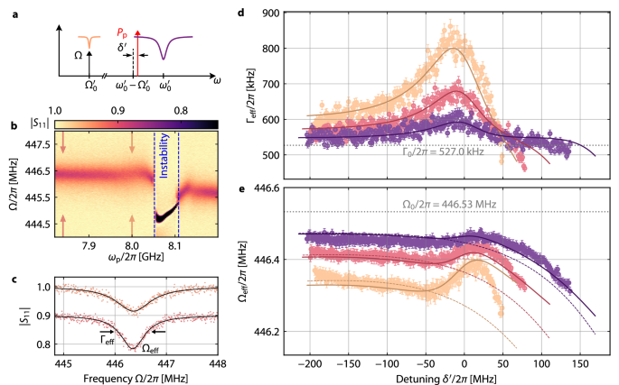
a Schematic of the experiment. A pump tone (red arrow) with frequency ωp and power Pp is applied around the red sideband of the HF mode. Detuning of pump from the red sideband is \(\delta^{\prime}={\omega }_{\mathrm{p}}-({\omega }_{0}^{{\prime} }-{\Omega }_{0}^{{\prime} })\). For each pair (ωp, Pp), the LF mode reflection is probed directly around \({\Omega }_{0}^{{\prime} }\) using the LF feedline and a VNA (black arrow). b Color-map of the LF reflection ∣S11∣ vs. pump frequency ωp. When the pump is far red-detuned from the HF mode red-sideband, the resonance is nearly unmodified compared to the pump-free case. Just below \(\delta^{\prime}=0\) or ωp/2π ≈ 8.0 GHz, the absorption gets wider and shallower and slightly shifts in frequency; both effects indicate dynamical backaction at work. Strikingly, for ωp/2π ≈ 8.05 GHz, which is still around the cavity red-sideband, a parametric instability region appears, which is experimentally identified by a strongly deformed resonance feature in S11, and the simultaneous disappearance of the HF mode in the HF reflection54. The two pairs of arrows indicate the linescans shown in c. Top curve in c shows ∣S11∣ at ωp/2π ≈ 8.0 GHz, the point of maximum photon-pressure damping, bottom curve is manually offset by − 0.1 for clarity and is for ωp/2π ≈ 7.84 GHz. Symbols are data, lines are fits, from which we extract Ωeff and Γeff. d, e Effective LF mode linewidth Γeff and effective resonance frequency Ωeff vs. detuning \(\delta^{\prime}\) for three different Pp, color code for Pp identical to Fig. 4, cf. Supplementary Fig. 15 for the corresponding nc. Symbols are data and error bars are standard errors obtained from the fit routine, lines are theory curves. Note the two clearest signatures for dissipative coupling: first, the maximum for the photon-pressure damping is at negative detunings from the red sideband. And second, for positive detunings from the red sideband the total damping rate is smaller than the intrinsic damping rate Γeff < Γ0, where Γ0 is shown as dashed line. This indicates negative backaction damping with a red-detuned pump, and is the precursor for the approaching parametric instability. To fully model the data, we included a cross-Kerr frequency shift to the LF frequency \({\Omega }_{0}^{{\prime} }={\Omega }_{0}+{{{\mathcal{K}}}}_{\mathrm{c}}{n}_{\mathrm{c}}\) with \({{{\mathcal{K}}}}_{\mathrm{c}}=2\pi \times -130.8\,{\mathrm{Hz}}\), and a small nonlinear cross-damping \({\Gamma }_{0}^{{\prime} }={\Gamma }_{0}+{\kappa }_{\mathrm{c}}{n}_{\mathrm{c}}\) with κc = 2π × 38.4 Hz. Dashed lines in e show \({\Omega }_{0}^{{\prime} }\).
A non-intuitive result of these experiments is that we observe a parametric instability, when the pump has a slightly higher frequency than \({\omega }_{0}^{{\prime} }-{\Omega }_{0}^{{\prime} }\), but is still far red-detuned. This is also predicted by theory, cf. Supplementary Note 6, and it is an intrinsic signature for the presence of dissipative coupling, which has also been studied in related optomechanical systems24,33. We can understand it from Eq. (10), which includes (for simplicity again in the sideband-resolved limit) that the photon-pressure damping \({\Gamma }_{\mathrm{pp}}={g}_{\omega }^{{\prime} 2}{\kappa }_{0}^{{\prime} }| \chi^{\prime}_{\mathrm{c}0} {| }^{2}+{g}_{\omega }^{{\prime} }{g}_{\kappa }^{{\prime} }\delta^{\prime} | \chi^{\prime}_{\mathrm{c}0} {| }^{2}\) has two contributions, the second of which changes sign with the pump detuning from the red sideband \(\delta^{\prime}={\omega }_{\mathrm{p}}-({\omega }_{0}^{{\prime} }-{\Omega }_{0}^{{\prime} })\) and is < 0 for \(\delta^{\prime} > 0\). So it enhances the dispersive PP damping for \(\delta^{\prime} < 0\), and counteracts it for \(\delta^{\prime} > 0\). In our case it even overcompensates it to \(\Gamma_{{\rm{eff}}} \le 0 \) (theoretical instability criterion) around \(\delta^{\prime} \approx+{\kappa }_{0}^{{\prime} }\) due to the large \(| {g}_{\kappa }^{{\prime} }/{g}_{\omega }^{{\prime} }|\) ratio for large nc. Similar considerations are valid for δΩpp. An additional signature for backaction interference is that the maximum of Γeff occurs at \(\delta^{\prime} < 0\), cf. Fig. 5d, instead of at \(\delta^{\prime} \approx 0\) as expected for \({g}_{\kappa }^{{\prime} }=0\). The slight shift of the maximum Γeff to lower frequencies with incressing Pp on the other hand reflects the increasing ratio \(| {g}_{\kappa }^{{\prime} }/{g}_{\omega }^{{\prime} }|\). A more detailed comparison between purely dispersive and mixed photon-pressure can be found in Supplementary Note 6.
To quantitatively model Γeff and Ωeff, we include also a cross-nonlinear damping and a cross-Kerr frequency shift, i.e.,
$${\Gamma }_{{\mathrm{eff}}}={\Gamma }_{0}+{\kappa }_{\mathrm{c}}{n}_{\mathrm{c}}+{\Gamma }_{\mathrm{pp}}$$
(12)
$${\Omega }_{{\mathrm{eff}}}={\Omega }_{0}+{{{\mathcal{K}}}}_{\mathrm{c}}{n}_{\mathrm{c}}+\delta {\Omega }_{\mathrm{pp}},$$
(13)
where both nonlinear effects are occurring naturally due to the constrictions being part of the LF mode in the galvanic coupling scheme. We fit the backaction data using all the HF mode and photon-pressure parameters obtained independently, and with the free parameters Γ0, Ω0, \({{{\mathcal{K}}}}_{\mathrm{c}}\) and κc. The cross-parameters we obtain from this are rather small with \({{{\mathcal{K}}}}_{\mathrm{c}}=2\pi \times -130.8\,{\mathrm{Hz}}\) and κc = 2π × 38.4 Hz, but the shift due to \({{{\mathcal{K}}}}_{\mathrm{c}}\) is still dominating the total pump-induced LF frequency shift. The cross-nonlinear damping on the other hand only contributes less than 10% to the deviations of Γeff from Γ0 at the maximum of Γeff, and the biggest part is due to Γpp. With the cross-nonlinearities included, we find good agreement between theory and data. The remaining deviations we attribute to uncertainties in the frequency-dependent pump-photon number, higher-order nonlinearities for the largest photon numbers and the onset of the parametric instability for the points close to the instability threshold. The recovery of the LF mode from the instability regime at ωp/2π ≳ 8.1 GHz, which is visible in Fig. 5b but not predicted by theory, is accompanied by the absence of the HF mode in the HF reflection54, which we believe is due to the pump photon number being so large that the cJJ SQUID is driven into the voltage state by overcritical peak HF currents. Overall though, the agreement between backaction data and model clearly confirms our above conclusions regarding Fano-like effects by dissipative coupling contributions and the nonlinearity-enhanced coupling rates, without which the datasets would lie much closer together for the pump powers used in Fig. 5d, e.