
Biodiversity impact calculations
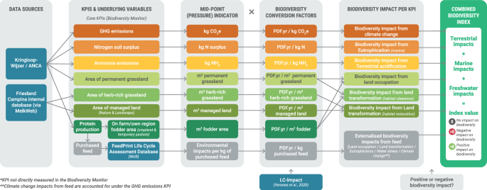
Our focal biodiversity metric is based on LCIA approaches, as is current good practice for comprehensive biodiversity footprinting (see e.g. ref. 7). The metric was based upon the KPIs monitored via the Biodiversity Monitor (see ‘Introduction’). Not only do these KPIs represent key pathways by which environmental pressures could impact biodiversity (e.g. GHG emissions, eutrophication); but they have also been agreed as relevant for DZK through a lengthy process of stakeholder engagement, and crucially, reflect data that are collected and therefore available to track long-term progress towards net biodiversity outcomes. To create a biodiversity index that integrated the KPI data (steps visualised in Fig. 1), conceptually, we:
1.
Gathered available KPI data (measures of environmental pressure) for the seven KPIs described in the Biodiversity Monitor, for all dairy farms in the Netherlands. Note that there are at least three additional possible KPIs not currently included in the Biodiversity Monitor which the authorship team felt could be relevant for incorporation into future iterations of the Biodiversity Monitor, but for which data are not currently available. These are pesticide use, water consumption, and phosphorus soil surplus;
2.
Treating each KPI as a ‘mid-point’ environmental pressure10, converted each KPI value into an estimate of biodiversity impacts using characterisation factors from the LC-Impact methodology. This was done at the level of KPIs for each individual farm—fully anonymised—to then be aggregated into a biodiversity impact per farm. Again, this is measured using the unit ‘Potentially Disappeared Fraction’ of species over time (PDF.year), which should be interpreted as an indicator for proportional contribution to global species extinction risk25. Here, PDF.year is used as a proxy indicator for combining and comparing biodiversity impacts across a range of mid-point pressures/KPIs; and,
3.
Summed PDF.year values across all farms to provide an estimate of biodiversity impacts over a given year for dairy production in the Netherlands.
We include the seven KPIs described in the Biodiversity Monitor: GHG emissions, nitrogen soil surplus, ammonia emissions, area of permanent pasture, area of herb-rich grassland, area of managed land (labelled ‘Nature & Landscape’), and ‘protein produced on own land/in farmer’s own region’ (Table 2). The raw data underpinning the KPIs was used e.g. the actual area of different land use types, CO2(e) value for GHG emissions, etc. (Fig. 1). ‘Protein produced on own land/in farmer’s own region’ is an indicator of the level of self-sufficiency (e.g., feed produced on own land), but is consequently indicative of the environmental footprint in other parts of the world (e.g., to grow ingredients like soy, used in concentrate feeds). To calculate the environmental impacts associated with purchased feed, we make use of the FeedPrint NL database developed by Wageningen University & Research, Blonk Consultants, and GFLI. KPIs were assumed to qualitatively correlate either positively or negatively with biodiversity impacts (e.g. the greater the emissions of GHGs, the more negative the impacts on biodiversity = negative correlation; Table 2).
Table 2 List of KPIs, with their potential for generating biodiversity gains
We note the following assumptions:
though the KPIs for ‘Nature & Landscape’ and ‘herb-rich grassland’ represent a range of different land management regimes (e.g., meadow bird management, landscape management, soil management, etc.), we treat them uniformly;
the biodiversity index is calculated by farm and then aggregated. We assume that biodiversity gains across all farms have equal weight, and do not, for example, consider any strategic spatial placement of biodiversity gains as part of core areas or corridors;
characterisation factors in LC-Impact24 are based on models that predict biodiversity losses per functional unit in terms of global species extinctions. To estimate biodiversity gains associated with certain activities e.g., Nature & Landscape management, we assume it is meaningful to apply these factors in reverse. This is a necessary assumption since, as far as we are aware, there are no comparable methods that model biodiversity gains from such a broad range of activities. Not only does this introduce some further uncertainty, but also we acknowledge that there is a temporal aspect here (in that reversing losses of biodiversity would likely take longer than causing it).
General data attributes
Data were available at farm-level for 14,686 farms in total, with values spanning the time period 2018–2020. Since 2020 was the only year for which comparable data were available across all of the KPIs collected under the Biodiversity Monitor, it was chosen as the baseline year. Data on the herb-rich grassland and Nature & Landscape KPIs were provided by Royal FrieslandCampina (RFC), with data on the remaining KPIs and contextual data provided from the KringloopWijzer (KLW) database. To convert KPI values into a biodiversity index value for the sector as a whole, we converted KPIs provided as relative values (e.g., kg CO2e per kg milk, or kg NH3 per ha) into total/absolute values per farm, by multiplying by either the total farm area or total milk production per farm. Datasets were matched based on unique farm identifiers, but all farms were anonymised.
Farms were excluded from the analysis if they did not report comprehensive data under the Biodiversity Monitor across KPIs, for land area, or on production. Similarly, farms were excluded if there were discrepancies between the total area reported for the farm, and for the different summed habitat components (e.g. for different grassland types across the KPIs). We note that there is a possibility that exclusion could lead to analytical biases in terms of the types of farms that had data gaps/mistakes, though this is not something we can assume. Since the relevant farms were those that by definition we could not calculate biodiversity impacts for, due to data gaps/mistakes, this is not something we analysed. Instead, we note this as a potential issue and an avenue for further research. After screening, the final dataset consisted of 8950 individual farms (62% of all dairy farms in the Netherlands, based on a total number of dairy farms recorded by CBS in 2020 of 14,54219).
For each farm, the total area of combined temporary grassland and cropland combined was estimated by subtracting the area of permanent grassland from the total area of the farm. Yard area was assumed to be minor, and so not considered in this analysis. Areas of grassland/cropland were then adjusted to account for areas provided for Nature & Landscape. These Nature & Landscape management areas provided in the RFC dataset were separated into four categories, based on the type of land the measure would be applied to (e.g., grassland, cropland, or landscape element—as per the Cumulatie and Grondgebruik table provided by Boerennatuur) and also based on the biodiversity weighting per management package, (provided in the Beheerpakketten Biodiversiteitsmonitor (BBM) documentation and associated appendices26,27). These categories are shown in Table 3. The distinction between these four categories was necessary for biodiversity index calculations, separating areas of low-intensity farming (which it is assumed would have a relatively low biodiversity impact compared to more intensive areas) from farmland habitats capable of generating absolute biodiversity gains. It was necessary to exclude some management packages from calculations in order to avoid double counting by area: specifically, BBM107 and BB107 (‘Bodemverbetering grasland met ruige mest’, ‘Bodemverbetering bouwland met ruige mest’, ‘Bodemverbetering met ruige mest’, ‘Chemie en kunstmestvrij land’) as they are applied in combination with other management packages.
Table 3 Categorisation of Nature & Landscape and herb-rich grassland areas
Since it was not always possible to determine from the dataset which land use types were overlapping (e.g., whether HRG was included under temporary or permanent grassland). The following assumptions were therefore made:
Area of HRG was subtracted from the total area of permanent grassland; and
Areas of low-impact grassland/arable land and Nature & Landscape areas were subtracted from the assumed arable/temporary grassland area. If these values exceeded the arable/temporary grassland area, the remainder was subtracted from permanent grassland areas.
While this involves making several assumptions, it was considered necessary and reasonable as a means to account for potential double counting of areas.
For the 2020 analysis, areas of land transformation/restoration were calculated using the change in area of herb-rich grassland or Nature & Landscape management per farm relative to the previous year (2019). This calculation was only made when data were available for both years, which was the case for 1237 farms for herb-rich grassland (14% of the dataset, 9% of all farms in the Netherlands), and 3753 farms for Nature & Landscape areas (42% of the dataset, 26% of all farms in the Netherlands).
Estimating environmental pressures associated with purchased feed
To estimate biodiversity impacts associated with purchased feed, we converted data provided on quantities of feeds into an estimated level of environmental pressure using the life cycle analysis (LCA) database FeedPrint (written consent was provided by the owners for this project). FeedPrint is also referred to in the calculation guidance for the KLW, particularly when calculating GHG emissions associated with feed, so we use FeedPrint as a consistent source for estimating all environmental pressures. FeedPrint provides ingredient- and country-level breakdown for a broad range of dairy feeds, and calculates the associated environmental pressures using the PEFCR-Feed methodology. We exported environmental data for feed components per country, with default parameters selected.
Data were provided for feed produced on the farms, and feed purchased by the farms. Feeds included concentrates, other roughage & by-products, maize, grass silage, and milk powder. It was assumed that the impacts of all feeds ‘produced’ by the farm were already accounted for by the other environmental KPIs (areas of grassland, total area of farm, N/NH3/CO2e emissions associated with growing fodder, etc.), so ‘produced’ feeds were excluded. Next, we assumed that ‘purchased’ grass and maize silage were produced on other farms within the Dutch dairy sector, and so were also excluded to avoid double counting.
Purchased concentrates and other roughage and by-products, however, were assumed to require additional analysis (i.e., produced by other sectors within the Netherlands, and/or by other countries). The analysis of purchased feeds therefore focuses on these two types of composite feeds.
To estimate the component ingredients in concentrates we used ‘concentrate dairy standard’ as a reference product, taking the ingredient and country-level breakdown directly from the FeedPrint database. ‘Other roughage & by-products’ is however a much broader category of feed ingredients; to determine constituent ingredients in this category, we referred to data published by Blonk Consultants28, which provided an in-depth life cycle inventory for Dutch semi-skimmed milk and semi-mature cheese. We referred specifically to Tables 3–10 of this report (using the most recent dry matter estimates provided within FeedPrint). The country-level breakdown for each of the composite ingredients was then sourced from FeedPrint, and can be viewed directly within the FeedPrint database software. Environmental values per kilogram of ingredient per country were exported for land occupation, freshwater eutrophication, marine eutrophication, and water consumption. Carbon values from FeedPrint were not used in order to avoid double counting, as these were assumed to be accounted for under the GHG emissions KPI (an assumption that follows KLW guidance).
While the area of land occupation is provided directly in FeedPrint, the area of land transformation (also known as land use change; LUC) is not. However, FeedPrint does provide estimates of carbon emissions associated with LUC, calculated using the PAS2050 methodology. Therefore, to calculate the area of LUC, we reverse this calculation using the same factors (provided in Annex C of the PAS2050:2011 guidelines). These factors are in the form of tonnes CO2e per ha per year, and are provided at local level for a set of countries. For countries not included in this list, we used the continental average.
The area of LUC was calculated for all feed ingredients except for those derived from soybean products. Soy was assumed to have no impacts associated with LUC due to the dairy sector’s requirement for sourcing 100% certified sustainable soy (RTRS or equivalent; see Table 1).
Calculation of biodiversity impact
There are several biodiversity metrics currently available for use in impact analysis, though none are widely accepted as standard. LCIA is an approach supported by leading frameworks (e.g. ref. 22), has precedent in the literature (e.g. ref. 29), and allows us to incorporate the full scope of environmental pressures (KPIs), converting these KPI ‘mid-points’ (pressures) into an estimated aggregated end-point impact on biodiversity.
LC-Impact software was chosen here because it is one of the most recently developed LCIA methodologies (developed as part of an EU FP7 project, via a collaboration between 14 partners). It incorporates spatial differentiation for environmental impacts where relevant, as well as levels of species vulnerability and endemism—both of which are lacking to some degree in other LCIA methodologies.
LC-Impact provides a set of characterisation factors (CFs), which can be used to calculate an estimate of biodiversity impact (in PDF.year) per unit of environmental pressure – for example, PDF.year per kg CO2e emitted, or PDF.year per m2 of land occupation. These CFs are based on a set of models from the scientific corpus that link the KPI to biodiversity via a particular ‘impact pathway’ (e.g., climate change, eutrophication, acidification, habitat conversion, etc.). Here, we mainly used the core set of CFs, using the marginal CF in the case of terrestrial acidification impacts linked to ammonia emissions; marginal CFs calculate the biodiversity impact of an additional kilogram of ammonia (as opposed to the average effect of a kilogram of ammonia). KPIs for CO2e emissions and NH3 emissions were combined directly with the relevant CFs. For other KPIs, further adjustments were made as follows:
Nitrogen soil surplus describes the balance between supply (e.g., from fertiliser, manure, fixation, etc.) and removal (e.g., via crops or emissions to air) of nitrogen compounds on farms. We ‘capped’ negative nitrogen soil surplus values at zero—assuming that net removals of nitrogen would be highly localised, and should not be accounted for when aggregating across farms—before combining values with the biodiversity CFs. We also note for completeness that the CFs for nitrogen model eutrophication are based on a commonly applied (e.g. ref. 30, assumption of nutrient limitation—that is: nitrogen is assumed to be the limiting nutrient in marine ecosystems and phosphorus is assumed to be the limiting nutrient in freshwater ecosystems. As such, the impact of nitrogen soil surplus is modelled in terms of eutrophication of marine systems (this takes into account a generic soil leaching fraction for the Netherlands and nutrient transport via river systems—see Verones et al.31 for more information) rather than of freshwater systems. This could lead to impacts from nitrogen soil surplus being underestimated in our metric—although there is evidence that phosphorus is a primary driver of freshwater eutrophication, including within the Netherlands (e.g. refs. 32,33,34), and that nitrogen limitation tends to be stronger in marine systems35. Furthermore, relatively low levels of phosphorus soil surplus are reported for Dutch dairy farms—which would translate into a biodiversity impact from freshwater eutrophication several orders of magnitude lower than other KPIs ( ~ 1.4 × 10−08 PDF.year, based on an average of 7 kg P2O5 recorded on the WUR Agro & Food portal). So, though we have used the best method available, we acknowledge that this is a simplified approach. There are high percentages of eutrophic freshwater bodies in the Netherlands36, which would ideally be improved by CFs that take into account site-specific nutrient limitation and synergistic effects of nitrogen and phosphorus37,38.
For land aspects, instead of applying the relevant factors provided via LC-Impact (based on a 2015 analysis), we substitute these for CFs calculated by Chaudhary and Brooks39. According to the authors of these resources, the 2018 factors are more up-to-date and reliable and can be directly substituted into LC-Impact. This also allows differences between three levels of land use intensity (minimal, light, intense) to be accounted for; definitions for each of the land use categories can be found in the supplementary material of Chaudhary and Brooks (2018). CFs for ‘light use’ pasture were applied to areas of permanent grassland, whereas CFs for ‘minimal use’ cropland and pasture were applied to areas of low-impact grassland/arable land. However, since ‘low-impact arable/grassland’ encompasses a broad range of management approaches with varying benefits for biodiversity, we also apply BBM weightings (see https://biodiversiteitsmonitor.nl/certificatie.html).
For herb-rich grassland or areas under Nature & Landscape measures: Any decrease in area was assumed to represent a loss of habitat, so we applied the CF for the Netherlands; conversely, the increase in area represented a gain, and we applied the CF in reverse. We acknowledge that using reversed CFs to estimate ‘biodiversity gains’ is not standard; however, it was necessary since, as far as we are aware, there are no comparable methods that model biodiversity gains from such a broad range of activities. As for low-impact arable/grassland (above), herb-rich grassland and different types of Nature & Landscape management have variable effects on biodiversity, which are reflected in the BBM weightings. To avoid these weightings overestimating biodiversity gains (the maximum possible proportional change in habitat restoration is 1 i.e., 100% habitat recovery), the weightings were normalised such that the maximum possible weighting was 1. Though this means that we effectively assume complete restoration for these areas, which would not happen in reality on short timescales, this is likely within the large uncertainty bounds for applying LCIA to biodiversity footprinting in any case24.
Areas undergoing LUC would also be associated with a change in GHG emissions; emissions associated with habitat loss, or sequestration through habitat restoration. We excluded GHG emissions from LUC linked to feed production, as those were already included within the values provided as part of the KLW dataset. Then, losses of habitat area were assumed to lead to an increase in GHG emissions, calculated using the values provided in Annex C of the PAS2050:2011 guidance. For any gains in habitat area (e.g., increases in herb-rich grassland or Nature and Landscape areas), GHG sequestration was estimated using the values provided by Table 3 of Schmidinger and Stehfest40, who calculate the average potential carbon sink per continental region and food product and provide factors in kg CO2/m2/year. GHG emissions and sequestration were both combined with the relevant CF in LC-Impact.
Accounting for other possible positive impacts
Passive restoration
Agricultural land released from productive use could, in the absence of action by other sectors, passively restore to natural habitat over time (e.g. ref. 41). In general, however, land released from dairy production was not assumed to deliver a biodiversity gain via passive restoration as it would likely be used for other purposes (i.e. outside of the dairy sector). This is consistent with the literature on the treatment of counterfactual scenarios in net outcomes policies for biodiversity (e.g. ref. 18). However, there could be cases in which land was set aside but still retained by dairy sector actors, and in that case, any passive restoration should be included in the overall calculations. Therefore, passive restoration of released land is included in our model in the specific scenario where total milk production remains the same or increases, alongside a reduction in land use. In such cases, we apply a high temporal risk multiplier to reflect the uncertainty in restoration timescales (see below).
Biodiversity offsets are measurable conservation outcomes (e.g., restoring species and habitats) that are widely used to compensate for residual negative impacts on biodiversity. We did not include offsets in our models here, as these are not currently a component of DZK strategy. However, offsetting could be included in future versions of our models—and we note that biodiversity gains linked to biodiversity restoration offsets would likely be needed as part of achieving net positive impact overall.
Applying multipliers to account for temporal risk for biodiversity gains
Time lags are important in conservation42. Impacts such as land use change may result in immediate biodiversity losses, but ecological gains from compensatory restoration activities may take time to accrue. Time lags are undesirable—particularly if species/habitats are threatened, or when the existence of biodiversity provides some ongoing ecosystem service that is diminished during the time lag.
A common approach is to apply a multiplier to areas being restored, in order to account for uncertainties around immediate/certain losses being compensated by delayed/uncertain future gains. The multiplier can be considered a ratio between damaged and necessary compensated amounts of biodiversity. It would be applied here as a factor to biodiversity gains, to calculate gains that account for these temporal uncertainties.
Laitila et al.23 propose a method to calculate minimum temporal multipliers associated with biodiversity restoration for offsets, which we apply to the biodiversity gains shown in Fig. 4 in the main text. Their method is based on the following parameters:
Time taken to restore different habitats (in number of years); The change in habitat condition (e.g., the proportional increase in biodiversity that is achieved by the restoration activity); A discount rate, which mathematically determines the currently perceived value of biodiversity gains that are not achieved until future years (‘net present value’); and, Permanence of the positive and negative impacts.
The values we applied for each parameter, for different restoration activities, are described in Table 4. The ‘permanence of impacts’ parameter was assumed to be 30 years for all habitats, being approximately equivalent to one generation (and therefore a feasible period of time for maintaining activities). Time lag values for habitat restoration are as advised by Meli et al.41 and via habitat management guidance provided by BoerenNatuur. Discount rates are as suggested by Overton et al.43. To calculate the change/improvement in habitat conditions associated with Nature & Landscape measures, we used the existing biodiversity weightings developed for the BBM and ANLb packages, which again were normalised as previously discussed.
Table 4 Parameters chosen for each of the three broad types of biodiversity restoration, and the final temporal multipliers calculated based on the tool/method provided by Laitila et al.23Biodiversity impact estimates for the full dairy production sector
After characterising all KPIs in terms of endpoint biodiversity impacts using the approaches described above, biodiversity impact values (in PDF.year) were summed across all farms (cf. Fig. 1). The total impact estimated for the filtered dataset was factored up to an estimate for the production sector as a whole, based on the total number of farms (14,54219), and total area under dairy production in 2020 (870,880 ha19).
Safeguard development
Setting any ‘net outcomes’ objective requires in part that any unavoidable biodiversity impacts are adequately compensated for (e.g., through biodiversity offsets). But to specify to what extent different biodiversity losses are permittable as part of net outcomes policies—and also in the context of uncertainties in calculating overall biodiversity impacts, as discussed throughout—we propose accompanying metrics with safeguards. These can be based both on empirical biophysical limits (at the level of the KPIs), as well as socio-political values. For example, a safeguard might specify that achieving net positive impacts on biodiversity should not be based on a strategy that includes deforestation of pristine rainforest through the Dutch dairy sector’s feed supply chain, or one that leads to levels of nutrient pollution within the Netherlands that are unhealthy for humans or wildlife. Further, strategies for biodiversity can be set at the level of safeguards on the relatively certain midpoint pressures (here, the KPIs) on the environment, and then monitored through the indicative if less certain endpoint biodiversity metrics.
It is unlikely that values can be maximised for all Biodiversity Monitor KPIs. For example, there may be farm-level trade-offs between KPIs (such as between protein produced on own land and nitrogen soil surplus, if production intensity is increased) or local constraints that limit performance. Safeguards help to define the safe operating space for the sector as a whole, allowing farm-level constraints and trade-offs to be navigated while striving for a genuine Net Positive impact on biodiversity at the sector level. Safeguards therefore need to be comprehensive enough to prevent perverse outcomes for nature, but practical enough to ensure feasibility when designing strategies towards a net positive target.
In developing safeguards here, we drew upon existing good practice guidance around achieving ‘net outcomes’ goals (such as net positive impacts on biodiversity), and associated topics (e.g. biodiversity offsetting). This includes peer-reviewed articles (e.g. ref. 6), business and financial institution standards and guidance (e.g., IFC Performance Standard 644, UK BNG Good Practice Principles), policy guidance (e.g., EU biodiversity strategy, Dutch Natuurpunten45), and stakeholder consultation sessions. These resources exhibit some common themes, which potentially serve as a good basis for determining categories of safeguards (Table 5).
Table 5 Proposed safeguard categories based on Net Positive Impact principles
During our research period, two stakeholder consultation meetings were organised. The objective of these consultations was not only to inform relevant stakeholders about the project but also to receive feedback on the proposed methodologies. The stakeholder consultation meetings took place virtually on December 6, 2021, and May 25, 2022 (running for 2 h in both cases). Where identified stakeholders were unable to attend the meeting, they were invited to provide feedback by email. Both consultations were hosted by the research team. Representatives from the following organisations participated in the stakeholder consultation:
Duurzame Zuivelketen (DZK)
IMAGEN
LTO
Staatsbosbeheer
Stichting Biodiversiteitsmonitor
Wageningen University & Research (WUR)
WWF France
WWF Netherlands (WNF)
The first consultation focused primarily upon the biodiversity metric, and the second consultation upon proposed safeguards. Separate documents outlining the status of methodologies were provided in advance of the meeting to attendees, and the research team presented research updates at each. Stakeholders asked questions, provided feedback, and made suggestions on how to improve the approach and methods. Finally, the project team hosted a focussed discussion about critical points where stakeholder input was essential to move forward with the project. All stakeholder inputs were recorded and evaluated, and incorporated into refinements to the methodology where relevant and appropriate.