
SLE details
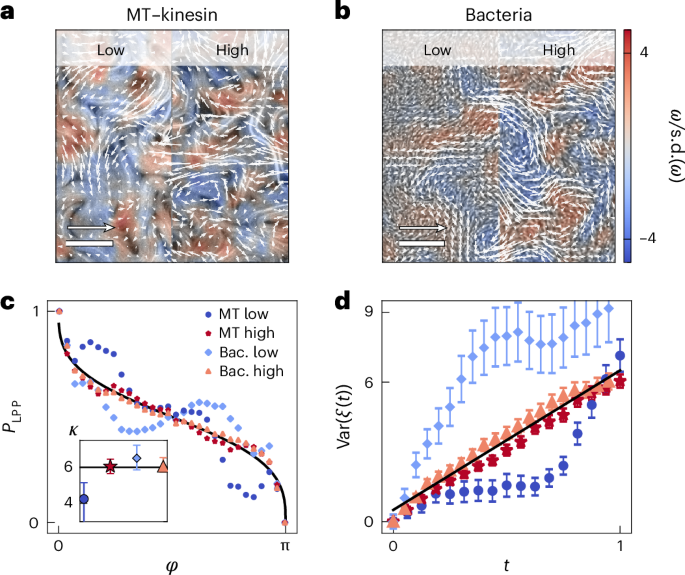
SLE is a one-parameter family of conformally invariant random curves14,15. The single parameter κ controls the fractal dimension of the curve, and specific values of κ correspond to the scaling limits of several well-known models: the loop-erased random walk with κ = 2 (ref. 17), the Ising model with κ = 3 (ref. 18) and critical percolation with κ = 6 (ref. 19). This makes SLE a powerful framework for identifying universality classes.
The Loewner equation describes the evolution of a conformal map gt in Loewner time t:
$$\frac{{\mathrm{d}}}{{\mathrm{d}}t}{g}_{t}(z)=\frac{2}{{g}_{t}(z)-{\xi }_{t}},\quad {g}_{0}(z)=z,$$
(2)
where ξ(t) is the driving function with Gaussian statistics 〈ξt〉 = 0, \(\langle {\xi }_{t}{\xi }_{{t}^{{\prime} }}\rangle =\kappa \delta (t-{t}^{{\prime} })\). The curve γ, known as the SLE trace, is traced out by those points satisfying gt(zc(t)) = ξt, where zc is the preimage of the real line.
By analogy with Brownian motion, κ acts as a diffusivity that determines the strength of driving in the Loewner equation. For κ = 0, the curve γ is a line with fractal dimension df = 1, whereas increasing κ makes γ progressively more winding or craggy until it fills the plane, reaching df = 2, according to the relation \({d}_{\rm{f}}=\min (2,1+\kappa /8)\) (ref. 59).
To determine κ and, thus, identify the universality class of our curves, we use two independent methods: the left-passage probability and the driving function.
Extracting candidate traces
To extract the nodal line (zero-vorticity isoline), we follow the standard procedure as in ref. 21. Starting from the vorticity field (Extended Data Fig. 1a), we binarize it as b = ω > 0, rotate by π/2 with a probability of P = 0.5 and set the origin at the centre of the lower boundary. At the domain edges, we assign value 1 for x < 0, and 0 otherwise (Extended Data Fig. 1b), ensuring that the trace starts at (x = 0, y = 0) and ends at (x = 0, y = L). An explorer is then initiated at the origin and follows the boundary between 0 and 1, keeping 1 to its left (Extended Data Fig. 1c).
Left-passage probability
The left-passage probability is defined as the probability that a point in the plane lies to the left of the SLE trace γ, that is, the curve passes to the right of a given point (Extended Data Fig. 2a). In other words, left passage means that there is a path from a point x on the real line with Re(x) < 0 to our test point, which does not cross the trace. It depends only on the polar angle φ from the curve’s origin, and the analytical form is known30 (equation (1)). We compare the measured left-passage probability for a set of points with cardinality S to the analytical prediction and extract κ through fitting. The mean square deviation Q(κ) is defined as
$$Q(\kappa )=\frac{1}{S}\sum _{z\in S}\frac{{(P(\varphi )-{P}_{\kappa }(\varphi ))}^{2}}{P(\varphi )(1-P(\varphi ))},$$
(3)
where P(φ) is the measured probability and Pκ(φ) is the theoretical distribution31,60. The reported diffusivity κ* corresponds to the minimum of Q(κ). The uncertainty range of κ is then defined by the set of κ ∈ K = [0, 8] values satisfying \({\mathcal{K}}=\{\kappa \in K| Q({\kappa }^{* })+\Delta Q({\kappa }^{* })\ge Q(\kappa )-\Delta Q(\kappa )\}\), where ΔQ is the measured uncertainty in the mean square deviation. The error bar is constructed as
$$\min {\mathcal{K}},{\kappa }^{* },\max {\mathcal{K}}$$
(4)
Driving function
A more direct method to determine κ is to measure the driving function ξt itself. We discretize Loewner time into steps ti with intervals Δi = ti − ti−1 and approximate ξt as constant within each interval, \({\xi }_{{t}_{i}}={\delta }_{i}\). We then apply the vertical slit map \({g}_{{t}_{i}}=\sqrt{{(z-{\delta }_{i})}^{2}+4{\Delta }_{i}}+{\delta }_{i}\) (Extended Data Fig. 2), which maps the vertical slit extending from δ to \(\delta +2i\sqrt{\Delta }\) onto the real axis, effectively ‘unzipping’ the trace γ (ref. 61). At each time step, we record the value of ξ, and by averaging over many realizations of γ, we obtain the trajectory of ξt. The diffusivity κ is then determined from the variance 〈ξ2(t)〉 = κt and verified by checking that ξt is Gaussian distributed.
Experimental detailsMicrotubule–kinesin system
Protein preparation
Stabilized microtubules were polymerized from heterodimeric (α, β)-tubulin purified from bovine brain (Biomaterials Facility, Brandeis University MRSEC) using a non-hydrolysable GTP analogue, guanosine-5-[(α, β)-methyleno]triphosphate (Jena Biosciences, NU-405), following a previously published protocol62.
A construct encoding the Drosophila melanogaster heavy-chain kinesin-1 fragment (Addgene ID: 15960) was expressed in Escherichia coli Rosetta (DE3), and recombinant kinesin protein was purified according to established protocols62.
Assembly of the active gel
Kinesin motor dimers were prepared by mixing biotinylated kinesin motor proteins with tetrameric streptavidin (Invitrogen, 434301) in a 2:1 molar ratio in the presence of 0.22-mM dl-dithiothreitol (Sigma-Aldrich, 43815). The mixture was incubated on ice for 30 min.
The dimerized motor complexes were then combined with a feeding solution containing ATP (Sigma, A2383), an ATP-regenerating system (phosphoenolpyruvate (Sigma, P7127) and pyruvate kinase/lactate dehydrogenase (Sigma, P0294)), the non-adsorbing polymer poly(ethylene glycol) (20 kDa) (Sigma, 95172) that promotes filament bundling through depletion, an oxygen-scavenging and antioxidant system (catalase (Sigma-Aldrich, C40), glucose oxidase (Sigma-Aldrich, G2133), d-(+)-glucose (Sigma-Aldrich, G7021), Trolox (Sigma-Aldrich, 238813) and dl-dithiothreitol) and the poly(ethylene glycol)-based triblock copolymer surfactant Pluronic F-127 (Sigma, P-2443).
Microtubules were added to the mixture immediately before the experiment. The final concentrations of all components are listed in Table 1.
Reactivation solution
Over time, the aqueous phase above the inactive active nematic layer at the water–oil interface accumulated enzymatic by-products. This liquid was exchanged with a fresh reactivation solution containing all components required for active gel preparation (Table 1), except microtubules. ATP was replaced with the NPE-caged ATP (adenosine 5′-triphosphate, P3-(1-(2-nitrophenyl)ethyl) ester and disodium salt) (Thermo Fisher Scientific, A1048) to allow the use of ultraviolet (UV) light to control the release of ATP available to the kinesin motors.
Active nematic cell
Experiments were performed in flow cells with a channel width of 1.5–2 mm, length of 15 mm and height of 150 μm. Each cell was assembled from superhydrophilic polyacrylamide-coated glass and superhydrophobic Aquapel-coated glass, separated by 150-μm-thick double-sided tape. Before coating, two holes of 1.5–2-mm diameter and 15-mm separation were drilled with a diamond wheel point (Dremel, 7134). These openings were later used for filling and exchanging the aqueous phase with the reactivation solution.
The cell was initially filled by capillarity with fluorinated oil (HFE7500, Fluorochem 051243) containing 2% fluorosurfactant copolymer (RAN Biotechnologies, 008 Fluorosurfactant). The active material was then introduced by capillarity, displacing the oil except for a thin lubricating layer. To prevent evaporation, the cell was sealed with petroleum jelly.
The active nematic layer formed at the water–oil interface and became inactive after about 24 h due to ATP depletion and accumulation of by-products. To reactivate the active nematic layer, the aqueous phase above the inactive layer was replaced with the reactivation solution. The petroleum jelly was temporarily removed to expose the channel openings. A drop of reactivation solution (two to three times the channel volume) was added to one hole, and a Kimwipes wiper (Kimtech, 34120) was inserted in the opposite hole to induce capillary flow. After replacement, the cell was resealed with petroleum jelly and illuminated with UV light (Thorlabs, M365LP1: 365-nm, 1,350-mW light-emitting diode) to release ATP from the NPE-caged ATP. Illumination was applied in pulses (2 Hz, 5% duty cycle, 8.09 mW cm−2) for 5 or 10 s. With this procedure, we first preform an active nematic layer at the water–oil interface. After losing activity, this layer preserves nematicity and maintains its integrity, at least over the timescales of the experiment. Following the exchange procedure with the reactivation solution, we released ATP from NPE-caged ATP in a controlled manner. This allowed us to study active nematic layer flows at extremely low activity levels, followed by a gradual increase in activity until fully developed active turbulence was achieved.
Imaging of the active nematic
Samples were imaged by fluorescence microscopy. Microtubule fluorescence was excited with a white light-emitting diode source (Thorlabs MWWHLP2) and a Cy5 filter set (Edmund Optics) and recorded using a charge-coupled device camera (ExiBlue, QImaging). Images were captured and processed using the open-source software μManager (ImageJ).
Image analysis
Raw experimental images were preprocessed in ImageJ and analysed using PIVlab in MATLAB to extract and quantify the velocity fields63.
Microtubule–kinesin activity estimation
In this section, we estimate the ATP concentration in the samples, allowing us to define the regions of low and high activity and to confine the conformal phase transition to activities in the interval [ATP]c ∈ (8, 18) μM.
We assume that UV illumination is spatially uniform across the entire experimental cell and that NPE-caged ATP is homogeneously distributed within the sample. Reflections of UV light from the output glass window back into the sample are neglected. To evaluate the activity of the active nematic layer, we estimated the concentration of ATP released after the photolysis of NPE-caged ATP as follows. The fraction of absorbed light, \({f}_{\rm{abs}}=1-1{0}^{-{\mathcal{A}}}\), was calculated from the absorbance of the reaction mixture, \({\mathcal{A}}\), using the Lambert–Beer law with the extinction coefficient for NPE-caged ATP, ε355 nm = 430 l mol−1 cm−1 (ref. 64). Then, to estimate the effective photocleavage of NPE-caged ATP, we first calculated the number of photons reaching the sample per second based on power measurements of UV light at the sample surface after transmission through the glass slide. To achieve this, the photodiode sensor (Thorlabs, S120VC) was positioned precisely at the sample location to maintain the geometrical fidelity of the illumination profile. The detector surface was covered with a glass slide, reproducing the optical interface present in experiments, and was exposed to identical incident power levels as those applied in the experiments. The number of photons reaching the sample per second was calculated as
$${N}_{\mathrm{photons}\mathrm{\,s}^{-1}}=\frac{P\frac{{A}_{\mathrm{cell}}}{{A}_{\det }}}{{E}_{356\mathrm{\,nm}}},$$
where P = 8.09 mW is the UV light power reaching the detector; Adet = 0.96 cm2 and Acell = 0.2625 cm2 are the areas of the detector and the experimental cell, respectively; and E356 nm = 5.446 × 10⁻¹⁹ J is the energy of a UV photon.
Using this value, the effective illumination time and the fraction of absorbed light, we estimated the number of absorbed photons. After correcting for the quantum yield of NPE-caged ATP, ϕ360 = 0.6 (refs. 64,65), we estimated the number of ATP molecules released and, thus, their concentration in the volume of the experimental cell.
The estimated ATP concentrations correlate with the mean enstrophy e obtained from particle image velocimetry (PIV) analysis: low-activity experiments occur below [ATP] ≈ 8 μM and e ≈ 2.8 ± 0.1 s−2, whereas high-activity experiments occur above [ATP] ≈ 18 μM and e ≈ 4.1 ± 0.4 s−2. The measured transition ATP concentration does not coincide with the increase in shear rate in microtubule–kinesin systems measured in ref. 66.
Bacterial suspension system
Dense suspensions of flagellar-propelled bacteria were confined within quasi-two-dimensional wells, where collective motion spontaneously emerged and evolved dynamically as oxygen was depleted. Bacillus subtilis (strain 168), a rod-shaped bacterium, was used as the self-propelled microswimmer.
Cells were revived from frozen glycerol stocks stored at −80 °C and inoculated into 10 ml of standard Luria–Bertani (LB) medium containing 1.0% tryptone, 0.5% yeast extract and 1.0% NaCl. Cultures were incubated overnight at 30 °C with shaking at 200 rpm. An aliquot of the overnight culture was then diluted into fresh LB to an initial optical density OD600 ≈ 0.05 and grown for 6–7 h to mid-exponential phase (OD600 ≈ 0.6). Cells were harvested at 3,000g for 5 min, washed twice with motility buffer (10-mM potassium phosphate, 0.1-mM EDTA, 10-mM NaCl, pH 7.0) and resuspended in the same buffer for experiments at a final OD600 ≈ 72. The typical bacterial body length was about 7 μm and diameter about 1 μm. Note that the bacterial volume fraction is only approximately estimated as ϕ ≃ 0.072, since an accurate determination is non-trivial. Typically, an optical density of OD600 = 1 corresponds to approximately 3 × 10⁸ bacteria per millilitre. Assuming a characteristic volume of ~1 μm3 per bacterium, this estimate yields a volume fraction on the order of 0.1%.
Quasi-two-dimensional confinement was achieved using a thin layer of polydimethylsiloxane (PDMS). A PDMS sheet of size 1 cm × 1 cm was patterned with an array of circular wells (diameter, 500 μm; depth, 10 μm). The PDMS wells were plasma treated to render them hydrophilic and able to hold the bacterial suspension. A 2-μl aliquot of concentrated bacterial suspension was deposited onto a treated coverglass and overlaid with the PDMS structure to form a sealed observation chamber. The assembled glass–PDMS construct was placed in a humidity-controlled environment with relative humidity above 90%.
Bacteria near the glass interface in the circular wells were imaged using a Nikon Ti2-E inverted microscope equipped with a ×60 water-immersion objective (numerical aperture 1.2) and a high-speed camera (Hamamatsu, ORCA-Flash4.0 V3, 1 pixel = 0.11 µm). As external oxygen was cut off, its concentration gradually decreased due to bacterial consumption, leading to a slow decay of collective activity. Videos were recorded every 5 min, with the first video starting at 3 min capturing the progressive loss of activity. Each recording was taken at 50 frames per second.
Bacterial activity estimation
Having found a transition between high and low activity in bacterial systems, we wanted to understand the transition point more quantitatively. Therefore, we compared our experiments to previous experiments on bacteria in which the oxygen levels were varied. Starting from the observation that the root mean square velocity Vr.m.s. measured by PIV decreases over time and that at some point during this process, SLE6 breaks, we wanted to understand how the activity changes in that time (Extended Data Fig. 4). Experiments on bacterial collective velocity, with controlled oxygen conditions, show that the relationship between oxygen concentration and collective velocity is linear34. We, therefore, compare our system with a system that has controlled oxygen levels. We note that our system starts at 25 °C and standard atmospheric pressure, leading to a concentration of oxygen in water equilibrated with air of 0.25 mM. Therefore, at t = 0 and oxygen concentration of 0.25 mM, we find \({V}_{{\rm{r.m.s.}}}(t=3\,\min )\approx 25\,\upmu {\rm{m}}\,{{\rm{s}}}^{-1}\) (Extended Data Fig. 4), which aligns well with previous results34. We then find that the activity drops with time, whereas time points \(3\,\min\) and \(5\,\min\) show SLE6 and time points \(10\,\min\) and \(15\,\min\) show broken SLE6. This means that the transition occurs between 12 μm s−1 and 21.7 μm s−1, which, comparing with ref. 34, corresponds to a transition at oxygen concentrations between 0.07 mM and 0.125 mM.
Model descriptions and computational detailsActive nematics
We use a standard active nematics model as described in refs. 3,33,67,68. We begin by defining a Landau–de Gennes free energy with bulk constant C and a Frank elastic term with elastic constant K in terms of the order parameter Q:
$${\mathcal {F}} =\int\!\!{\rm{d}}\mathbf{r}\,C(1-\mathrm{Tr}({{{Q}}}^{2}))\mathrm{Tr}({{{Q}}}^{2})+\frac{K}{2}{({\rm\nabla }\cdot {{Q}})}^{2}.$$
(5)
From this free energy, we derive the molecular field \({{H}}={\left(\frac{\delta {\mathcal{F}}}{\delta {{Q}}}\right)}^{\mathrm{ST}}\), which is the symmetric and traceless (ST) part of the functional derivative of the free energy with respect to the order parameter Q.
The dynamics of Q are governed by its relaxation towards the free energy minimum and by its coupling to the flow field \(\bf{u}\):
$$\frac{D{{Q}}}{Dt}-{{S}}=-\frac{1}{\gamma }{{H}},$$
(6)
where \(D/Dt={\partial }_{t}+\bf{u}\cdot \nabla\) is the material derivative. The corotation term \({{S}}=(\lambda {{E}}+\Omega )\cdot ({{Q}}+{{I}}/2)+({{Q}}+{{I}}/2)\cdot (\lambda {{E}}-\Omega )-2\lambda ({{Q}}+{{I}}/2)({{Q}}:{\nabla }\mathbf{u})\), with \({{E}}=\frac{1}{2}({\nabla }\mathbf{u}+{({\nabla }\mathbf{u})}^{\!\top })\) and \(\Omega =\frac{1}{2}({\nabla }\mathbf{u}-{({\nabla }\mathbf{u})}^{\!\top })\) representing the rate of strain and the vorticity tensors, respectively, controls how the nematic field responds to gradients in the flow \(\bf{u}\) with the flow alignment parameter λ. The rotational viscosity γ sets the rate of relaxation towards equilibrium.
The flow field \({\bf{u}}\) obeys the incompressible Navier–Stokes equations
$$\frac{D\mathbf{u}}{Dt}=\nabla \cdot {{\varPi }},\quad \nabla \cdot \mathbf{u}=0,$$
(7)
where the total stress is given by Π = Πviscous + Πpassive + Πactive. The viscous stress is Πviscous = 2ηE, and the passive stress combines pressure and elastic contributions as
$$\begin{array}{ll}{\varPi }_{ij}^{\,\text{passive}\,}=-p{\delta }_{ij}+2\lambda ({Q}_{ij}+{\delta }_{ij}/2)({Q}_{lk}{H}_{kl})\\\qquad\qquad\;-\lambda {H}_{ik}({Q}_{kj}+{\delta }_{kj}/2)-\lambda ({Q}_{ik}+{\delta }_{ik}/2){H}_{kj}\\\qquad\qquad\;-{\partial }_{i}Q_{kl}\frac{\delta {\mathcal{F}}}{\delta {\partial }_{j}Q_{lk}}+{Q}_{ik}{H}_{kj}-{H}_{ik}{Q}_{kj}.\end{array}$$
where p denotes the pressure. The active stress Πactive = −ζQ injects energy into the system through the orientational order. The activity parameter ζ, therefore, tunes the strength of non-equilibrium driving.
Fluctuating active nematics
To separate the effects of explicit activity from those of stochastic forcing, we use a fluctuating nematic model introduced in ref. 35. This model modifies the standard active nematic equations by replacing the deterministic active stress with stochastic noise, resulting in the following equations:
$$\frac{D{{Q}}}{Dt}-{{S}}=-\frac{1}{\gamma }{{H}}+{{{\xi }}}^{\,Q},$$
(8)
$$\frac{D{{\bf{u}}}}{Dt}=\nabla \cdot {{\varPi }}+\nabla \cdot {{{\xi }}}^{\,u}.$$
(9)
Again, H is the molecular field and γ is the rotational viscosity, whereas the stress Π remains the same as in the active nematic model but without the active term. The noise terms ξQ and ξu are Gaussian and have zero mean. Their variances are given by
$$\left\langle {\xi }_{ij}^{Q}(\mathbf{x}, t){\xi }_{kl}^{Q}({\mathbf{x}}^{{\prime} },t^{{\prime} })\right\rangle =\displaystyle\frac{2}{\gamma }{k}_{\rm{B}}{T}_{Q}{{\mathcal{J}}}_{ijkl}\delta (\mathbf{x}-{\mathbf{x}}^{{\prime} })\delta (t-{t}^{{\prime}}),$$
(10)
$$\left\langle {\xi }_{{ij}}^{u}(\mathbf{x},t){\xi }_{{kl}}^{u}({\mathbf{x}}^{{{{\prime} }}},{t}^{{{{\prime} }}})\right\rangle =2{k}_{{\rm{B}}}{T}_{u}\eta { \mathcal J }_{{ijkl}}\delta (\mathbf{x}-{\mathbf{x}}^{{{{\prime} }}})\delta (t-{t}^{{{{\prime} }}}),$$
(11)
with position x and time t, where kB is the Boltzmann constant and η is the solvent viscosity. The tensor \({{\mathcal{J}}}_{ijkl}={\delta }_{ik}{\delta }_{jl}+{\delta }_{il}{\delta }_{jk}-{\delta }_{ij}{\delta }_{kl}\) ensures that fluctuations preserve the symmetry and tracelessness of Q and the symmetry of the stress tensor.
The strengths of the nematic and fluid fluctuations are controlled by TQ and Tu, respectively. As there is no active term involving ζ, the model is explicitly passive when TQ = Tu, because detailed balance is preserved. However, detailed balance is broken when TQ ≠ Tu, allowing the system to behave as an effectively active fluid driven by stochastic forcing. This framework provides a clean way to test whether conformal invariance arises from general non-equilibrium fluctuations rather than specific microscopic mechanisms. In our analysis, we compare the geometric statistics of zero-vorticity contour lines for both fluctuating passive (TQ = Tu) and fluctuating active (TQ ≠ Tu) regimes.
Computational implementation of nematic models
All simulations of active fluid models are performed using a hybrid lattice Boltzmann approach68, with the implementation of fluctuations following refs. 35,69.
The simulations are carried out in a periodic square domain of side length L = 2,048. The system is initialized with a small amount of noise n0 in the nematic order parameter field to avoid metastable states. Each system is first equilibrated until the number of defects reaches a steady state, where applicable.
The parameters listed in Table 2 correspond to a low-Reynolds-number regime, with Re ≈ O(10−1).
Comparison of critical percolation and active nematics
To fully show the similarities between the cluster boundaries in critical percolation and the vorticity nodal lines in active nematics, we show examples of both lines and compare them using the yardstick method, which measures their fractal dimension.
We find that in both cases, the traces are visibly scale free (Extended Data Fig. 5a,b), with the difference that although the critical percolation trace has a small range cut-off set by the lattice spacing, for active nematics that cut-off is set by elasticity and is, therefore, somewhat longer. This is also visible in the measure of the fractal dimension (Extended Data Fig. 5c), where both curves follow N(L) ≈ L−7/4 but the crossover into that regime is at a higher value of L for the active nematic trace, leading to the offset between the curves.
Conformal transition in fluctuating active nematics
To test the necessity of active driving, we use the fluctuating nematic model in equation (9) in which by tuning the nematic fluctuations and flow fluctuations, TQ and Tu, respectively, we can break detailed balance by setting TQ ≠ Tu, or conserve detailed balance when TQ = Tu (ref. 35). We, therefore, test whether the transition to fully developed active turbulence is a genuinely active phenomenon that arises from detailed balance breaking.
For different values of the reduced distance from equilibrium, u = (TQ − Tu)/(TQ + Tu), such that u = 0 is at equilibrium and u = 1 is maximally distant from equilibrium, we first measure whether the systems exhibit scale-free contour lines with a fractal dimension df = 7/4, as expected for SLE6 (ref. 59). We measure the fractal dimension df using the established yardstick method in which the contour is measured with yardsticks of different lengths L to determine the scaling of the required number of sticks \(N(L) \sim {L}^{-{d}_{\rm{f}}}\) (refs. 27,70).
When the system is at equilibrium u = 0, we find a simple scaling in the nodal lines (zeros of the vorticity field) N ≈ L−1, corresponding to regular curves. As we increase the non-equilibrium driving u, the system transitions to a scale-free regime with N ≈ L−7/4, consistent with SLE6 (Extended Data Fig. 6a).
To test for conformal invariance, we next measure the winding angle ϕ, which is known to scale with contour length s as \({\rm{Var}}(\phi )=(6/7)\log (s)+c\) for SLE6 curves71,72. We define the winding angle ϕ as follows. Discretizing the curve into straight line segments indexed by i, each pair of consecutive line segments i and i + 1 meets at an angle αi, where α = 0 if the segments are parallel (Extended Data Fig. 2b). The total winding angle of a curve of length s is then calculated as \(\phi (s)=\mathop{\sum }\nolimits_{0}^{s}{\alpha }_{i}\). We find that when u is large and the system is active, Var(ϕ) follows the expected SLE6 scaling, whereas at lower u, it deviates from this behaviour (Extended Data Fig. 6b). The winding angle of a conformally invariant curve must also be Gaussian distributed71, which we confirm for high u (Extended Data Fig. 6b, inset).
Although the left-passage probability is inconclusive in this system, probably because domain-spanning interfaces are rare and the assumptions of the chordal SLE geometry are not strictly satisfied, the driving function measurements show SLE6 behaviour for active systems (not shown).
We, therefore, find that for equilibrium fluctuating nematics (TQ = Tu), all measures deviate from SLE6, demonstrating that activity and detailed balance breaking are required to reach the fully developed active turbulence phase.
Geometric and mechanical percolationDetection of vortex centres
To locate the centres of rotational flow structures, we computed the discrete winding number m of the velocity field v = (vx, vy) (ref. 36). Grid points satisfying the topological condition ∣∣m∣ − 1∣ < ε (with ε = 0.3) were identified as candidate vortex centres.
We then applied a geometric refinement based on the local flow structure. For each candidate, the velocity field within a radius of three grid points was decomposed into radial and tangential components. A defect was accepted as a vortex centre only if the tangential kinetic energy contributed more than 75% of the total local kinetic energy (Eθ/Etot > 0.75).
Weak excitations were filtered out by requiring the vorticity magnitude at the defect centre to exceed the spatial standard deviation of the vorticity field:
$$| \omega | > {\sigma }_{\omega }.$$
(12)
The sign of ω indicates the rotation direction of the vortex (+1 for clockwise rotation and −1 for counterclockwise rotation). Detections within three grid spacings were merged to yield a single vortex centre per coherent structure. A representative snapshot is shown in Extended Data Fig. 7a.
Geometric percolation
To quantify the geometric connectivity among vortex centres, we performed a percolation analysis using random geometric graphs37,38. For each snapshot, the set of N vortices located at positions {xi} were treated as nodes in a graph. Two vortices i and j were connected if their Euclidean separation was smaller than a probing threshold r.
We computed the percolation order parameter P∞, defined as the fraction of vortices belonging to the largest connected cluster:
$${P}_{\infty }(r)=\frac{1}{N}{\mathop{\max }\limits_{k}}| {s}_{k}(r)| ,$$
(13)
where ∣sk∣ is the size of the kth cluster. To compare systems at different activity strengths ζ, the probing distance r was normalized by the characteristic length ℓ = r(gmax), extracted from the peak of the pair correlation function g(r) (Extended Data Fig. 7b).
By gradually increasing r/ℓ, we tracked the growth of the largest connected component (Extended Data Fig. 8a shows a schematic) and identified the effective percolation threshold rc as the point at which P∞ = 0.5 (Extended Data Fig. 8b).
Mechanical percolation
To characterize the mechanical rigidity of the vortex network, we constructed a graph in which neighbouring vortices were connected according to the alpha-shape complex39,40 with parameter α = 2ℓ. Rigidity was then analysed using the pebble game algorithm23 following ref. 25. This graph-theoretic method decomposes the network into rigid and floppy regions by testing whether each added bond introduces an independent constraint or a redundant one, thereby identifying maximally rigid clusters23,41.
For each configuration, we calculated the fraction of all vortices belonging to the largest rigid cluster, fLR, which serves as the order parameter for rigidity percolation.
Persistent homology
The inputs to our persistent homology calculations are the vorticity field, \(\omega={\nabla }\times \mathbf{u}\). From these, we compute the SEDT field, which encodes how far a given point is from a domain the sign of the vorticity of which is opposite (or equivalently, the zero-vorticity contour line). This transformation is sketched in Extended Data Fig. 9c. The computed distance is (arbitrarily assigned to be) negative for points inside the domains with negative vorticity. We normalize these distances by the active length scale, which we estimate to be \(\sqrt{K{\zeta }^{-1}}\). Table 2 lists the details on these quantities.
Using standard tools in topological data analysis and persistent homology42,43,44, we compute persistence diagrams from these distance-transformed fields using the sublevel-set method. In effect, we flood the SEDT field and measure how the topology changes during this process, noting birth and death of features as the flood level increases (Extended Data Fig. 9).
We note that due to vorticity being a pseudo-vector, the choice between the super- and sublevel methods is (also) arbitrary. Persistence diagrams are then a way of showing the results of the filtration. An example of the first persistence diagram is shown in Extended Data Fig. 9d. In these diagrams, a topological feature is denoted by its birth and death (b, d), which are the values of the sublevel set for which the feature appears and disappears.
Thus, for the regular landscape shown in Extended Data Fig. 9a, the persistence diagram would have a very narrow distribution, up to point-like for a sine landscape, whereas for the rougher landscape shown in Extended Data Fig. 9b, the persistence diagram will be much more widely distributed. The zeroth persistence diagram captures the emergence and disappearance of connected components in the sublevel sets of our field; thus, each topological feature corresponds to a minimum in the field (and the birth is the value of the field in that minimum), and the death of such a topological feature is the value for which the component ‘merges’ with another. For the first persistence diagram, we encode the behaviour of the closed loops that emerge during the sublevel-set filtration. In the first diagram, the birth is the first sublevel set for which a given loop is found, and its death is the value for which the loop closes or merges with another.
We visualize the general trend across our simulation by depicting the persistence p = d − b, and plot their distributions (Extended Data Fig. 10, p > 3). Below the critical activity, the simulations stabilize vorticity domains with specific dimensions, as evidenced by the bimodality of the distributions. Once ζ crosses the critical threshold, the distributions shown in Extended Data Fig. 10 cease to be bimodal and transition to long-tailed distributions reminiscent of those refined from Gaussian random fields73.
To capture this phenomenon in a quantitative manner across the different values of ζ, we convert these persistence diagrams into persistence images46 (Extended Data Fig. 9e shows an example) using a Gaussian kernel (with width σ = 4) weighted by the expression \(\arctan \left(c{(d-b)}^{n}\right)\) (with c = 10−5 and n = 3) and subject these to principal component analysis to extract the general trends in the data across the different levels of activity. These parameter choices are the result of a systematic search, and provide the optimal distinction of the states of our system. Although the persistence diagrams, which capture the lifetimes of all features, clearly show a difference between low- and high-activity active nematics, the use of principal component analysis on the persistence images allows us to reduce the dimensionality of the persistent homology results and, therefore, crystallize the transition activity in this analysis. These results agree very well with the transition activity measured with the other methods.