A split attractor design for rapidly writing a navigational goal

Fly stocks

Female flies were raised on standard cornmeal-agar medium at 25 °C on a 12-h light cycle. For optogenetics experiments, the food was supplemented with 50 µl of 35 mM all-trans retinal (Sigma, R2500, dissolved in ethanol) mixed with ~1 teaspoon of hydrated potato flakes. Experimental flies were aged to 1–3 days for electrophysiology experiments or 9–14 days for imaging experiments. A list of fly genotypes is shown in Supplementary Table 2 and a list of fly reagents is shown in Supplementary Table 3.

Two-photon calcium imaging

Calcium imaging was performed as described in our previous study26. In brief, we anaesthetized flies over ice and a chilled (4–10 °C) aluminium sarcophagus and then glued them onto custom 3D-printed holders. We minimized movement of the brain by stabilizing the proboscis and head, and glueing the eyes, head and anterior tip of the thorax to the holder. To access the FB for imaging, we removed a small piece of the surface cuticle, trachea and air sacs over the back of the brain using sharpened forceps. We positioned flies over an air-supported ball (9 mm diameter General plastics FR-7110, painted with black spots, supported by 0.4 l s−1 air) using two cameras (30 fps, FLIR Blackfly, Computar 8.5 mm 1:1.3 adjustable lens) at the front and side of the fly. A third camera (100 fps, Grasshopper, 94 mm/0.5× InfiniStix Proximity Series lens, Edmund Optics Focal Length Extenders, working distance 15 cm) was used to track the ball using Fictrac software70. We illuminated the fly and ball using two infrared LEDs (M850F2) and T-cube LED Drivers (LEDD1B) coupled to fibre optic cables (Thorlabs M118L03 flat cleave patch cables). We continuously perfused (1 ml min−1) the brain with extracellular saline (103 mM NaCl, 3 mM KCl, 5 mM TES, 8 mM trehalose dihydrate, 10 mM glucose, 26 mM NaHCO3, 1 mM NaH2PO4H2O, 1.5 mM CaCl22H2O and 4 mM MgCl2.6H2O, pH 7.1–7.4, osmolarity 270–274 mOsm) bubbled with carbogen (5% CO2, 95% O2) and warmed to 33 °C.

We performed all imaging under a 20× water objective (Olympus Plan Fluorite XLUMP 20×/1.0) using an infrared laser (SpectraPhysics MaiTai HP or Coherent Axon 920) at 920 nM and 25–35 mW (measured at sample) using a galvo-galvo scanner. Simultaneous fluorescence emission from GCaMP7f and tdTomato were separated by bandpass filters (Semrock, FF01-525/50-32 for green and FF01-607/70-32 for red) and detected using two GaAsP photomultiplier tubes. We captured volumes consisting of three 192 × 96 µm optical sections, separated by 15 µm, taken at 8 volumes s−1 with a 1.2 µs dwell time.

In all imaging experiments, flies walked on a floating ball and received wind (25 cm s−1) and odour (0.5% apple cider vinegar, 0.3 l min−1) stimuli controlled by custom Python code. The wind direction was set by a rotary union (Dynamic Sealing Technologies, LT-2141-OF-ES12-F1-F2-C2) controlled by a stepper motor (Oriental PKP566FMN24A, with controller CVD524-K) and microcontroller (TeensyDuino +USB), and was controlled in closed loop by the flies’ heading measured by ball movement as we described previously26. The starting wind direction was randomly selected from 0°, 45°, −45°, 135° or −135°. Wind was on from 5–60 s of each 65 s trial. The odour signal was randomly selected between five possible patterns on interleaved trials: odour step (15 s) or odour pulses of 1, 4, 7 or 10 pulses (1 Hz, 0.5 s pulse width). When the odour was turned off, a compensatory air valve was opened to maintain total air speed. Air to all lines (wind, ball support, odour, compensated air) were passed through a pressure regulator (Cole-Parmer MIR2NA) and charcoal filters (Drierite 26800 Drying column, with desiccant replaced by activated charcoal). Wind and compensated air were also humidified. Airflow for the wind line was controlled by a mass flow controller (Aalborg Model GFC17), while airflow for odour, compensated air, and ball support were controlled by flowmeters (Cole-Parmer PMK1-010608). We controlled the timing of wind stimuli using a solenoid valve (Cole-Parmer Masterflex 01540-11), and the timing of odour and compensate using high-speed three-way solenoid valves (Lee company, LHDA1233115HA).

During wind-shift experiments, the wind was rotated by 90° across 2.2 s either in the presence of odour (10 pulses at 1 Hz) or without odour. The onset of the shift was set to occur 4 s after odour onset. We also included control trials where wind was not shifted in the presence or absence of odour. The data from non-shift control trials were included in all analyses that did not depend on the precise odour stimulus.

Electrophysiology

For electrophysiology, we anaesthetized flies over ice, glued them to custom 3D-printed holders, and then removed their two front legs. To access dorsal cell bodies, we removed a large piece of the cuticle, trachea, and air sacs from the back of the brain, then manually detached the sheath using fine forceps. We minimized brain movements by removing the muscles on the brain and stabilizing the proboscis with glue. Starting at the dissection, and maintained throughout the entire experiment, we continuously perfused extracellular saline (same recipe as above), bubbled with carbogen, over the brain. Using a 40× objective (Olympus, LUMPLFLN40XW), an LED source (Cairn Research MONOLED), and a filter (U-N19002 AT-GFP/F LP C164404) we visualized GFP-positive cell bodies for recordings. Prior to recording, we cleaned the area around the target cell using fine-tip glass pipettes filled with extracellular saline.

For patch clamp recordings, we pulled glass pipettes with a Sutter P-1000 puller, pressure polished the pipettes (final resistance of 3–5 MΩ), and then filled them with intracellular solution (140 mM KOH, 140 mM aspartic acid, 10 mM HEPES, 1 mM EGTA, 1 mM KCl, 4 mM MgATP, 0.5 mM Na3GTP, and 13 mM biocytin hydrazide). We amplified the voltage signals using an Axonpatch 200B amplifier with a Brownlee Precision 410 preamplifier and then digitized the signals at 10 kHz. We delivered 73 µW mm−2 red light (625 nm, measured at light source) for activating CsChrimson using a Thorlabs LED (M625F2) and T-Cube LED Driver (LEDD1B) coupled to optical fibres cables (Thorlabs M118L03 flat cleave patch cables) positioned below the head.

To better observe a mixture of excitation and inhibition, we depolarized cells to −38.1 ± 7.1 mV (mean ± s.d., n = 37 cells) using a small amount of positive current. Cells that did not spike were discarded. In all experiments, we randomly looped through 11 stimuli: seven optogenetic light stimuli (4 s of 12 µW mm−2 low power; 4 s of 23 µM mm−2 medium power; 4 s of 73 µM mm−2 high power; 1 Hz pulses with 0.2 duty cycle; 1 Hz pulses with 0.5 duty cycle; 1 Hz pulses at 0.8 duty cycle; and a light plume stimulus), three current stimuli (4 s of −4 pA; 4 s of 0 pA; and 4 s of 4 pA), and one wind or odour stimulus (wind on for 20 s, 5% apple cider vinegar on for 4 s). We constructed the light plume stimulus by filtering the odour encounters of a fly navigating in a virtual olfactory plume26 with a positive derivative filter. The stimuli were looped five times in all cells, and then five times per drug condition. While we only report the results of light pulse stimuli in this paper, the voltage changes we observed—such as fast inhibition or slow persistent excitation—were seen across all optogenetic temporal patterns used.

In several experiments, we perfused drugs onto the brain to block neurotransmitter receptors. In these experiments, drugs were mixed with extracellular saline and perfused onto the brain for at least five minutes before resuming stimulus presentation. Since picrotoxin generated large excitatory responses to synaptic input, we often hyperpolarized the cells to −50.3 ± 10.2 (mean ± s.d., n = 10 cells) to minimize depolarization block. If cells did enter depolarization block, we paused the experiment until the cell recovered. The list of drugs, their sources and the final concentrations used are listed in Supplementary Table 4.

Immunohistochemistry

To perform immunohistochemistry, dissected brains were fixed in 4% paraformaldehyde (dissolved in PBS) for 15 min, washed 3× in PBS, incubated in 5% normal goat serum (dissolved in PBST) for 60 min, incubated overnight in primary antibody solution (dissolved in 5% normal goat serum), washed 3× in PBST, incubated overnight in secondary antibody solution (dissolved in 5% normal goat serum), washed 3× in PBST, and washed 3× in PBS. The primary antibody solution contained chicken anti-GFP (Fisher Scientific RRID:AB_1074893) 1:50, mouse anti-nc82 (DSHB RRID:AB_2314866) 1:50, and rabbit anti-dsRed (Clontech 632496) 1:500. The secondary antibody solution contained Alexa488-conjugated goat anti-chicken (Fisher Scientific RRID:AB_2534096) 1:250, Alexa633-conjugated goat anti-mouse (Fisher Scientific RRID:AB_2535719) 1:250, and Alexa568-conjugated goat anti-rabbit (Fisher Scientific RRID:AB_2576217) 1:250. For imaging, the brains were mounted on microscope slides, immersed in Vectashield (Vector Labs H-1000), sealed with coverslips, and then imaged using a 20× objective (Zeiss W Plan-Apochromat 20×/1.0 DIC CG 0.17 M27 75 mm) on a Zeiss LSM 800 confocal microscope at 1.25 μM depth resolution.

To compare hemibrain neuron morphology to R65C03-GAL4 (Extended Data Fig. 2c), we warped a stain of R65C03 (from Flylight71) and hemibrain skeletons of layer 6 tangential neurons using the 2018 Janelia female template brain72. We overlaid the warped stain and warped skeletons and identified neurons with high overlap.

Data analysisConnectomic analysis

Data from the hemibrain connectome16 were obtained from neuprint explorer (http://neuprint.janelia.org, hemibrain:v1.2.1) and analysed using custom Python code. Prior to visualizing the weight matrices (Fig. 5a and Extended Data Fig. 1f), we sorted each cell type by their FB or protocerebral bridge x position (that is, columns), with h∆K positioning determined by their axons. To count the fraction of FB6M or FB5V synapses onto h∆K axons, we sorted synapses by their x position on a h∆K cell-by-cell basis. To calculate the ratio of recurrent synapse to EPG synapses (Extended Data Fig. 9b), we also examined data from the FAFB (https://codex.flywire.ai, FAFB v783) and male CNS (http://neuprint.janelia.org, male-cns:v0.9) connectomes. For each PFG neuron, we calculated the total number of synapses from h∆K neurons, the total number of synapses to h∆K neurons, and the total number of synapses from EPG neurons. The recurrence was the average synapses to and from h∆K neurons, and this was divided by the total inputs from EPGs to calculate the ratio. Since the FAFB data was less curated, and occasionally contained PFG neurons with 0 connectivity to EPG or h∆K neurons, we only included PFG cells that had a total recurrence strength and heading strength both above 10. Neuron and brain visualizations in Extended Data Fig. 1a,b were made using Flywire data17,73 in Codex (https://codex.flywire.ai/?dataset=fafb&data_version=783)74.

Calcium imaging and behaviour analysis

We used fictrac software70 to transform the x, y and z rotations of a custom-made ball into 2D walking trajectories. The forward velocity and angular velocity were directly calculated as rotations around the x and z axes, respectively, which were then used to calculate heading (motor position, calculated as the integral of angular velocity), position (x = integral of forward velocity × sin(heading); y = integral of forward velocity × cos(heading)), and upwind velocity (vy = forward velocity × cos(heading)). The rotation around the y axis (side velocity) was additionally used to calculate travel direction (heading + tan−1(forward velocity/side velocity)). For data analysis, the position, angular velocity, angular speed, upwind velocity, and forward velocity were smoothed using a running average of 1 s width.

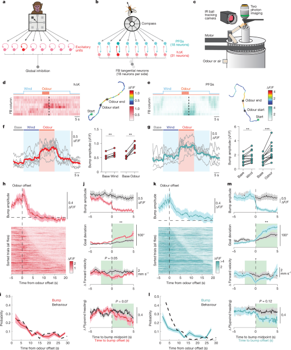
We used custom Matlab software to pre-process our calcium imaging data (see ref. 26 for details), including motion correction, fluorescence extraction (across eight hand-drawn regions of interest (ROIs) across the FB), and alignment with fictrac behavioural data. To detect activity bumps in h∆K neurons, PFG neurons, and neurons labelled by VT062617-Gal4, we lowpass filtered bump amplitude data (Butterworth filter (sampling rate (fs) = 100 Hz, cut-off frquency (fc) = 2 Hz)) and then established a threshold on a trial-by-trial basis according to the minimum ∆F/F value of that trial and the ∆F/F s.d. across all trials. For most analyses, this threshold was set at minimum(∆F/F) + 1 × s.d., but to identify large PFG bump onsets and offsets for Fig. 1k–m, the threshold was increased to minimum(∆F/F) + 1.75 × s.d. A minimum bump duration was set at 3 s, and any above-threshold activity within 3 s of bumps was merged. To calculate bump position, the raw ∆F/F values across all 8 ROIs were smoothed (running average, width ~2 s) and then fit with a von Mises distribution at each time step using the Matlab function fminsearch. To aid fitting, we used the previous bump position or the ROI with the maximum ∆F/F (if the previous time step did not have a bump) as the initial search values. These bump positions were reported as a phase angle, where −180° is the left side of the FB and 180° is the right side of the FB.

During calcium imaging of FB5V and FB6M neurons, the calcium signal showed an artefactual decay from trial start to trial end. This artefact was removed by fitting an exponential decay using the beginning (first 5 s) and end (last 5 s) of the ∆F/F signal, and then subtracting this fit from the ∆F/F signal. Therefore, all ∆F/F signals reported for FB5V and FB6M are changes from this baseline.

In Fig. 1i,l, and Extended Data Fig. 1k, we calculated the persistence of walking direction following odour. To calculate the persistence of walking direction, we first defined a goal direction as the mean heading direction adopted in the first second after odour offset (post odour) or after trial start (baseline control), and then identified the time when flies stopped walking (forward velocity under 0.5 mm s−1 for at least 1.5 s) or deviated from the goal direction by at least 45°. In Fig. 1h,i,k,l, we calculated the persistence of neural activity following odour. To calculate the neural persistence, we calculated the time between odour offset and bump offset. To better compare neural and behavioural persistence, we only considered trials where the bump activity turned on before odour offset and turned off after odour offset.

In Fig. 1j,m, we aligned bump amplitude and behavioural data to bump offset. We only included trials where the bump activity turned on before odour offset and turned off after odour offset, and we removed any data before bump onset. In control bump ON data, we took the same trials, but only included data between bump onset and bump offset, each aligned by the midpoint of the bump. For goal deviation, the ‘goal’ was defined as the mean heading during the first 1/6th (between 0.18 and 4.46 s) of the bump ON or bump offset data. The durations of bump ON and bump offset data were matched for each trial.

In Fig. 3d, we calculated the mean bump width of h∆K activity. To do this, we isolated periods with bumps, aligned the raw ∆F/F calcium signals (across 8 ROIs) to the column with the highest signal, and then normalized the activity by the maximum activity.

In Fig. 4d, we calculated the maximum bump deviation and cumulative bump deviation. To quantify maximum bump deviation, we calculated the difference between the minimum and maximum unwrapped bump position between each bump onset and offset. To quantify cumulative bump deviation, we calculated how much the unwrapped bump position changed at each time point between bump onset and offset, summed the absolute value of these changes, and then divided the sum by the total length of the bump period.

In Fig. 4e–g and Fig. 6f,g,o,p, we identified discrete periods of turning. To identify turns, we identified segments of data where the unwrapped heading shifted by at least 90°. We then identified the beginning and end of each turn by searching backwards or forwards in time, respectively, until the heading stabilized (the maximum change in heading over 0.25 s was smaller than the 80th percentile of heading s.d. across all bins of the same duration). Since this algorithm isolated periods of turning with different durations, when turns were aligned in time (Figs. 4g and  6f,o), the data were time warped such that all turns were equal in length. In cases where small turns were compared to large turns (Fig. 4g), turns were classified as small if the total change in heading was less than 130°, and large otherwise.

In Fig. 4e,f, we further classified behaviour as ‘rest’ or ‘straight running’. Rests were defined as periods of low movement (v < 0.5 mm s−1) for at least 3 s. Straight running was defined as movements with high walking speed (v > 50th percentile of speed for given fly) and stable heading (∆heading < 90°). Short straight running bouts (under 3 s) within 1 s of larger bouts were merged, and large bouts (over 3 s) within 3 s of each other were merged. Any turns that had overlapping sections with straight running bouts were removed.

In Fig. 4h, we calculated discrete shifts in h∆K bump position following turns. To do this, we identified pairs of h∆K bumps separated in time. For each bump pair, we calculated the change in wrapped heading from the end of the first bump to the beginning of the second bump, and then classified the pairs as left turns (0° > ∆heading) or right turns (0° < ∆heading). Since these data were wrapped, we centred the wrapping around the bump position or heading taken at the end of the first bump.

In Fig. 4i–k, we selected trials where a bump was present for the entire duration of the wind-shift stimulus and the fly walked for at least 20% of the bump period. We then calculated the rotational gain across these bump periods by dividing the cumulative change in unwrapped bump position by the cumulative change in unwrapped heading. Therefore, each data point in Fig. 4i represents a single bump from a single wind-shift trial. As both bump position and heading are represented by angles (see above for bump position), a rotation gain of 0 indicates stable bumps and a rotation gain of 1 indicates perfect tracking. The average bump amplitudes were calculated across the same time periods as the rotational gains. We ensured that the bump position and heading data were pre-processed equivalently by filtering both data sets using the same filters (moving average with a width of 13 samples at 100 Hz) and downsampling the data to match the original imaging sampling rate (downsample from 100 Hz to 6.37 Hz). To test the robustness of the correlation between bump amplitude and rotation gain, we bootstrapped the data (with replacement) 10,000 times and calculated s.d. error on the fit, R2 and P values. For Fig. 4k, we analysed all trials that contained an odour stimulus. For each time point, the rotation gain was calculated by comparing the cumulative change in bump position to the cumulative change in heading within a 2 s window beginning at that timepoint. To avoid timepoints where the bump was mostly absent or the fly heading was stationary, we excluded timepoints if the total window did not contain sufficient bump data (<50%), if the cumulative delta heading was too low (<0.4°), or if the rotational gain was too high (>5).

In Extended Data Fig. 8b–f, we correlated bump position with heading or travel direction for each trial. We only excluded trials if the trial contained no bump activity.

In Fig. 6e,n, we cross-correlated FB5V and FB6M ∆F/F signals with angular speed or upwind velocity. Prior to cross-correlating, we mean subtracted the fluorescent and behavioural signals. To remove wind-coupled activity fluctuations in FB6M data, we only used data from 5 s after wind onset and 5 s before wind offset.

In Fig. 6h,q, we aligned FB6M and FB5V activity to deviations from goals. We first defined a goal direction as the mean heading adopted in the first second after odour offset, and then aligned neural and behavioural data to the time when flies deviated from this goal by at least 45°.

Electrophysiology analysis

For analysis of electrophysiology data, the voltage traces were lowpass filtered using a Butterworth filter (fs = 10,000 Hz, fc = 5 Hz), downsampled by a factor of 10, and then baseline subtracted. We calculated persistent excitation (Fig. 2d,f,i and Extended Data Fig. 3e,h) by summing the baseline-subtracted voltage signal between light offset and trial end, and then normalizing by the length of this period. For visualizing voltage signals across trials (for example, Fig. 2c), the voltage signals were sorted by persistent excitation (Fig. 2a,c,e,g,h and Extended Data Fig. 3a) or inhibition during the stimulus (Fig. 2j,l and Extended Data Fig. 4c).

Statistics and reproducibility

All statistics were ran using GraphPad Prism 10 and reported in Supplementary Table 1. Non-parametric statistical tests were used if the data were not normally distributed (see Supplementary Table 1). An alpha value of 0.05 was used to determine significance, with *0.01 < P < 0.05, **0.001 < P < 0.01, ***0.0001 < P < 0.001, ****P < 0.0001 reported on figures. For imaging experiments, flies were only included for further analysis if they reliably oriented upwind on at least 50% of trials, which was identified by a convergence of heading values towards the upwind direction (0°) and an increase in mean upwind velocity around wind or odour onset. For electrophysiology experiments, cells were only included for analysis if they showed visible spiking activity, defined as rapid deflections above 10 mV. Other than these criteria, all data and replications were included in the manuscript. Sample sizes (number of flies or cells) were selected based on previous experiments. Stimuli were randomized within each experiment. Experimenter was not blind to genotype but all analyses were applied programatically to all datasets without regards to genotype.

ModellingFull FB model

To model the FB recurrent network, we created a rate-based dynamical system model consisting of 30 h∆K neurons, 18 PFG neurons, and 1 global inhibitory neuron. We approximated all dynamical systems using Euler’s method of integration with a time step of 0.001 s. To generate ring recurrence between h∆K and PFG neurons, we gave each neuron a relative position in the FB, indicated by an angle from 0 to 2π, and then connected the populations with local excitation that was maximum at overlapping positions and decayed with distance. This was done explicitly using a Gaussian equation fit to the real connectivity from the hemibrain connectome (Figs. 3 and  5) or using the connectivity directly from the connectome (Extended Data Fig. 6). The local spread of the Gaussian connectivity was set by the local connectivity width (σ, Gaussian s.d.), which establishes how quickly the connectivity decays as the distance (in radians) between h∆K and PFG neurons increases (σPFG>h∆K = 0.25, σh∆K>PFG = 0.25, in radians). The best fit Gaussian connectivity was found by searching for the local connectivity width (σ) that minimized the absolute error between the fit weight matrix and real weight matrix. Each column of the real weight matrix (the connectivity of each PFG neuron to all h∆K neurons) was normalized to ensure fits were based on the local connectivity width rather than variability in synaptic strength across the FB. Although real h∆K neurons have a 180° shift across the FB, for simplicity, we only show connectivity and activity simulations from the ‘axons’ of h∆K neurons. The weight matrices between h∆K or PFGs and the global inhibitory neuron were either one-to-all or all-to-one. To simulate the neural activity of each population, we used the following ordinary differential equations:

$${\tau }_{{\rm{h}}\Delta {\rm{K}}}\times \,\frac{{\rm{d}}{\vec{u}}_{{\rm{h}}\Delta {\rm{K}}}}{{\rm{d}}t}=-{\alpha }_{{\rm{h}}\Delta {\rm{K}}}\times {\vec{u}}_{{\rm{h}}\Delta {\rm{K}}}+{\mathrm{exc}\times W}_{\mathrm{PFG},{\rm{h}}\Delta {\rm{K}}}{\vec{U}}_{\mathrm{PFG}}-{W}_{\mathrm{inh},{\rm{h}}\Delta {\rm{K}}}{\vec{U}}_{\mathrm{inh}}+{\vec{I}}_{{\rm{h}}\Delta {\rm{K}}}$$

(1)

$${\tau }_{\mathrm{PFG}}\times \frac{{\rm{d}}{\vec{u}}_{\mathrm{PFG}}}{{\rm{d}}t}=-{\alpha }_{\mathrm{PFG}}\times {\vec{u}}_{\mathrm{PFG}}+{\mathrm{exc}\times W}_{{\rm{h}}\Delta {\rm{K}},\mathrm{PFG}}{\vec{U}}_{{\rm{h}}\Delta {\rm{K}}}-{W}_{\mathrm{inh},\mathrm{PFG}}{\vec{U}}_{\mathrm{inh}}+{\vec{I}}_{\mathrm{PFG}}$$

(2)

$${\tau }_{\mathrm{inh}}\times \frac{{\rm{d}}{\vec{u}}_{\mathrm{inh}}}{{\rm{d}}t}=-{{\alpha }_{\mathrm{inh}}\times \vec{u}}_{\mathrm{inh}}+{\mathrm{inh}\times (W}_{{\rm{h}}\Delta {\rm{K}},\mathrm{inh}}{\vec{U}}_{{\rm{h}}\Delta {\rm{K}}}+{W}_{\mathrm{PFG},\mathrm{inh}}{\vec{U}}_{\mathrm{PFG}})+{\vec{I}}_{\mathrm{inh}}$$

(3)

Where \(\tau \)x is the time constant for population x, αx is the leak of population x, \(\vec{u}\)x is the activity of population x, exc is the excitation strength, inh is the inhibition strength, Wx,y is the weight matrix from population x to population y, \(\vec{U}\)x is the synaptic output of population x, and \(\vec{I}\)x is the external input to population x. \(\tau \)x and \(\alpha \)x were set to 1 and 10, respectively, for all populations. \(\vec{I}\)x was used to set the input patterns to each population.

To simulate the synaptic output of each population, we used the following second-order ordinary differential equations to simulate alpha functions:

$${{\vec{U}}_{x}}^{{\prime\prime} }=-({a}_{x}+{b}_{x})\times {\vec{U}}_{x}^{{\prime} }+{a}_{x}\times {b}_{x}\times ({F}_{x}({\vec{u}}_{x})-{\vec{U}}_{x})$$

(4)

Where 1/ax is the decay rate of the alpha function for population x, 1/bx is the growth rate of the alpha function for population x, and Fx is the activation function of population x. The synaptic growth and decay values used for fast and slow synapses were fit to synaptic physiology data by searching for the a and b values that minimized the absolute error between the fit activity and synaptic physiology voltage data. The fast synapses were fit to h∆K voltage responses to FB6M (49B08AD; VT063626DBD) pulsed stimulation, and were set to ax = 4.63 and bx = 25. The slow synapses were fit to h∆K voltage responses to FB6A/D (65C03-Gal4) stimulation in the presence of curare (10 µM) and IMI (100 nM), and were set to ax = 0.64 and bx = 25. We used the following activation functions:

$${F}_{{\rm{h}}\triangle {\rm{k}}/\mathrm{PFG}}({u}_{x})=\left\{\begin{array}{c}0\,\mathrm{if}\,{u}_{x} < 0\\ {u}_{x}\,\mathrm{if}\,{0 < u}_{x} < 1\\ 1\,\mathrm{if}\,{u}_{x} > 1\end{array}\right.$$

(5)

$${F}_{\mathrm{inh}}({u}_{x})=\left\{\begin{array}{c}0\,\mathrm{if}\,{u}_{x} < 0\\ {u}_{x}\,\mathrm{if}{0 < u}_{x}\end{array}\right.$$

(6)

During the simulations in Fig. 3, sinusoidal (direct offset = 1), Gaussian (normalized such that max = 1), or random input (Gaussian distribution with µ = 1, σ = 0.5) were provided to the h∆K and PFG neurons for 4 or 10 s. During the simulations in Fig. 5 and Extended Data Figs. 8a and  9e, we only provided input to PFG neurons, which was sinusoidal with a phase that we randomly and stochastically updated over time. Phase shifts were stochastic, occurring with a 0.1% chance at each time step, and when they occurred, they were randomly drawn from a Gaussian distribution with µ = 0 and σ = 50° and then smoothed over time according to:

$${\tau }_{\mathrm{smooth}}\times \frac{{\mathrm{dheading}}_{\mathrm{smooth}}}{{\rm{d}}t}={\mathrm{heading}}_{\mathrm{raw}}-{\mathrm{heading}}_{\mathrm{smooth}}$$

(7)

Where \(\tau \)smooth equals 1. To account for the differences in synaptic strength between EPGs>PFG and h∆K<->PFG synapses, we decreased the amplitude of the sinusoidal input to 1/6 of the recurrent excitation strength. We controlled the gate in Fig. 5 by either externally changing the excitation strength (exc in equations (1,2), increased from 0 to 7) or changing external input to h∆K (\({\overrightarrow{I}}_{{\rm{h}}\Delta {\rm{K}}}\) in equation (1), inhibition corresponded with a value of −5, and disinhibition corresponded with a value of 0). In Extended Data Fig. 9e, we additionally attempted to gate bump dynamics by adding external input to h∆K and PFG neurons (\({\overrightarrow{I}}_{{\rm{h}}\triangle {\rm{K}}}\) and \({\overrightarrow{I}}_{\mathrm{PFG}}\) in equation (1), increased from −1 or −2 to 0).

To calculate the network decay rate in Fig. 3, we calculated the maximum difference in h∆K output at each time step following external input offset and then fit this difference with an exponential decay function.

In Fig. 3d, we expanded the model simulations to predict how each simulation would appear if the neurons were recorded using population imaging, such as calcium imaging. Calcium imaging captures activity throughout each active neurons’ axons. Therefore, we calculated how much each model neuron should spread across the FB to synapse with its postsynaptic partners. This spread was then applied to the model simulation to get a better prediction of how far activity of the active neurons would spread across the FB. In Extended Data Fig. 5f,g, to keep the neuron size the same across simulations we used real connectome data to estimate the width of real h∆K neurons, and then used this spread to estimate the width of FB activity. We fit the relationship between local connectivity s.d. and FB activity percentage with an exponential equation.

In the parameter space in Extended Data Fig. 7c,d, for each pair of parameters (ainhibition and aexcitation), we first calculated the decay tau of the excitatory neuron across each excitatory strength value, removed all values above 30 s, and then we summed these values to get the total ‘sum’.

In Fig. 5f and Extended Data Fig. 6, we calculated the bump position by finding the relative position (as an angle) of the neuron with the maximum activity.

Simple recurrent network model

To simplify the recurrent network to two dynamic variables, we began by reducing the h∆K and PFG populations to one global excitatory neuron. This led to the following 6 variable dynamical system:

$${\tau }_{\mathrm{exc}}\times \frac{{\rm{d}}{u}_{\mathrm{exc}}}{{\rm{d}}t}=-{u}_{\mathrm{exc}}+{W}_{\mathrm{exc},\mathrm{exc}}{U}_{\mathrm{exc}}-{W}_{\mathrm{inh},\mathrm{exc}}{U}_{\mathrm{inh}}+{I}_{\mathrm{exc}}$$

(8)

$${\tau }_{\mathrm{inh}}\times \frac{{\rm{d}}{u}_{\mathrm{inh}}}{{\rm{d}}t}=-{u}_{\mathrm{inh}}+{W}_{\mathrm{exc},\mathrm{inh}}{U}_{\mathrm{exc}}+{I}_{\mathrm{inh}}$$

(9)

$${{U}_{\mathrm{exc}}}^{{\prime\prime} }=-({a}_{\mathrm{exc}}+{b}_{\mathrm{exc}})\times {{U}_{\mathrm{exc}}}^{{\prime} }+{a}_{\mathrm{exc}}\times {b}_{\mathrm{exc}}\times ({F}_{\mathrm{exc}}({u}_{\mathrm{exc}})-{U}_{\mathrm{exc}})$$

(10)

$${{U}_{\mathrm{inh}}}^{{\prime\prime} }=-({a}_{\mathrm{inh}}+{b}_{\mathrm{inh}})\times {{U}_{\mathrm{inh}}}^{{\prime} }+{a}_{\mathrm{inh}}\times {b}_{\mathrm{inh}}\times ({F}_{\mathrm{inh}}({u}_{\mathrm{inh}})-{U}_{\mathrm{inh}})$$

(11)

We made two simplifying assumptions. First, we assumed that the synaptic rise and decay constants (1/ax, 1/bx) were much slower than the membrane time constants (\(\tau \)x). This means that the variables uexc and uinh instantaneously follow the synaptic dynamics. Second, we assumed that the synaptic decay time constant (ax) was much slower than the synaptic rise time constant (bx). These assumptions lead to the following two-variable dynamical system:

$${{U}_{\mathrm{exc}}}^{{\prime} }={a}_{\mathrm{exc}}\times ({F}_{\mathrm{exc}}({W}_{\mathrm{exc},\mathrm{exc}}{U}_{\mathrm{exc}}-{W}_{\mathrm{inh},\mathrm{exc}}{U}_{\mathrm{inh}}+{I}_{\mathrm{exc}})-{U}_{\mathrm{exc}})$$

(12)

$${{U}_{\mathrm{inh}}}^{{\prime} }={a}_{\mathrm{inh}}\times ({F}_{\mathrm{inh}}({W}_{\mathrm{exc},\mathrm{inh}}{U}_{\mathrm{exc}}+{I}_{\mathrm{inh}})-{U}_{\mathrm{inh}})$$

(13)

We used the same activation functions as those used for the excitatory and inhibitory neurons in the full model (equations (5,6)). During simulations, we kept Wexc,inh constant at 1, whereas we varied Wexc,exc and Winh,exc with excitation strength and inhibition strength, respectively. During input, the excitatory unit received an external input equal to 1, whereas the inhibitory unit received no input.

Reporting summary

Further information on research design is available in the Nature Portfolio Reporting Summary linked to this article.