
Laser set-up
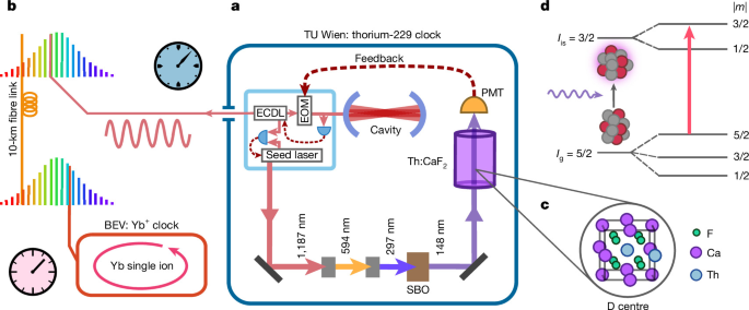
In the 229Th interrogation system, a commercial laser (FHG-TA Pro, TOPTICA) provides an output power of approximately 500 mW at a wavelength of 296.8 nm, frequency-quadrupled in two doubling stages and one amplification stage from a diode seed laser at 1,187 nm. The final second-harmonic-generation process is based on nonlinear frequency conversion in an SBO crystal kept under a high-purity N2 atmosphere (purity 5.0). Fundamental radiation still present in the beam after the final second-harmonic-generation step is separated using three dielectric-coated mirrors. For the absorption measurements, we used a head-on type PMT (R6835, Hamamatsu) mounted inside the vacuum chamber and operated at 2.5 kV. We used the same segment of the X2 sample60 as in ref. 7. The segment in use has a cylindrical geometry with a diameter of 3.1(1) mm and a length of 4.2(1) mm and was oriented such that the beam traversed along the centre line of the piece. The measured average concentration of 229Th in the segment was 6.6(5) × 1015 mm−3.
The seed laser of the FHG-TA was locked to the clock laser (CLS, TOPTICA) through an offset frequency phase lock. A fast photodiode with a bandwidth of 10 GHz measured the beat frequency between the two lasers, which was then mixed with a reference frequency. The fast loop of this lock actuated on the seed laser diode current, and the slow loop was used to steer the grating of the laser diode. The laser was scanned by modulating the reference frequency.
Like the actuators of the offset lock, the Pound–Drever–Hall lock of the clock laser to the cavity was also configured such that the fast feedback loop actuated on the laser diode current, whereas the slow feedback signal of the Pound–Drever–Hall scheme controlled the position of the grating for optical feedback to the laser diode.
For clock comparison measurements and drift rate measurements of the cavity, the beat frequency fb of the clock laser with the frequency comb (FC1500-250-ULN, Menlo) was recorded using a dead-time-free frequency counter (K+K FXE) operated in Π-type counting mode61,62 at a gate time of 1 s. Our method of comparing the thorium clock at TU Wien with the Yb+ clock (TOPTICLOCK, TOPTICA)63 at BEV follows the scheme described in ref. 7. The Yb+ clock was based on the 435.5-nm E2 transition of a single 171Yb ion.
All frequency synthesizers and counters in the 229Th clock system and the frequency comb were referenced to the 10-MHz signal of a commercial Rb clock (FS725, SRS).
To perform an absorption measurement at a specific frequency, we modulated (square wave) the offset lock frequency between the seed laser diode and the clock laser with 10 Hz between the target frequency and an off-resonance frequency. Each modulation cycle was also reflected in a synchronization signal connected to a time-resolved pulse counter (TimeTagger Ultra, Swabian Instruments). The modulation ensured that power fluctuations in the laser output did not affect the measurement. The detection set-up consists of a PMT, a radiofrequency amplifier and the pulse counter, which binned the arriving pulses from the PMT relative to the last synchronization edge. The absorption was then calculated by subtracting the on-resonance counts from the off-resonance counts and dividing by the off-resonance counts.
Clock operation
To operate the set-up as a clock, we first acquired a single absorption spectrum, as shown in Extended Data Fig. 2a. We observed that a Lorentzian line shape fits our absorption measurement data well. We then measured the expected error signal (Extended Data Fig. 2b). To measure an error signal, we modulated the offset lock frequency with 10 Hz between two frequencies flow and fhigh. The difference Δf = fhigh − flow was kept constant during the measurement, and only the centre was swept across the resonance. In our measurements, we used a frequency deviation Δf of \({f}_{{\rm{FWHM}}}/\sqrt{3}\), with fFWHM describing the FWHM of the measured absorption peak (Extended Data Fig. 2a). We fitted this signal with the function
$${y}_{{\rm{f}}{\rm{i}}{\rm{t}}}(f)=\frac{{A}_{{\rm{L}}}}{1+{\left(\frac{f+\Delta f/2}{\gamma }\right)}^{2}}-\frac{{A}_{{\rm{L}}}}{1+{\left(\frac{f-\Delta f/2}{\gamma }\right)}^{2}},$$
where AL is the amplitude and γ is the half width at half maximum of the Lorentzian. For the clock operation, the laser frequency was again switched between two frequencies while we adjusted the centre position with the feedback. For both frequency positions, the counts clow,i and chigh,i were recorded, where i is the measurement index for averaging the signal. The applied error signal E can be calculated as
$$E(c)={y}_{{\rm{fit}}}^{-1}\left(\frac{1}{L}\mathop{\sum }\limits_{i=1}^{L}\frac{{c}_{{\rm{high}},i}-{c}_{{\rm{low}},i}}{({c}_{{\rm{high}},i}+{c}_{{\rm{low}},i})/2}\right),$$
with the number of cycles L and the inverse fit function \({y}_{{\rm{fit}}}^{-1}(c)\). Extended Data Fig. 2c illustrates an adjustment step inferred by the calculation of E. With the integration times set in the clock operation, the beat was shifted after every interrogation cycle by the calculated value E, as shown in Extended Data Fig. 1.
Variation of the fundamental constants
The variation of α(t) relates to the variation of the ratio of the 229Th and ytterbium clock frequencies through: \(({k}_{\mathrm{Th}}^{\alpha }-{k}_{\mathrm{Yb}}^{\alpha })\times {\partial }_{t}\,\log \,\alpha (t)\,=\) \({\partial }_{t}\,\log ({f}_{\mathrm{Th}}/{f}_{\mathrm{Yb}})\). Here \({k}_{{\rm{Th}}}^{\alpha }\) and \({k}_{{\rm{Yb}}}^{\alpha }\) are sensitivity factors that describe how much the respective transition frequency depends on α. The log-derivative directly corresponds to the measured infrared beat frequency fb through \({\partial }_{t}\log ({f}_{\mathrm{Th}}/{f}_{\mathrm{Yb}})=8({\partial }_{t}\,{f}_{{\rm{b}}})/{f}_{0}\), where the factor of 8 originates from the three frequency-doubling steps64.
The anomalously low energy of the 229Th nuclear transition arises from a coincidental near-cancellation of the mega-electronvolt-scale strong force and Coulomb contributions to the binding energies of the nuclear states involved15. We, therefore, expect that \({k}_{\mathrm{Th}}^{\alpha }\approx {k}_{\mathrm{Th}}^{{\rm{g}}}\approx {k}_{\mathrm{Th}}^{{m}_{q}}\), where \({k}_{{\rm{Th}}}^{g}\) and \({k}_{{\rm{Th}}}^{{m}_{q}}\) are the sensitivity constants that relate between the log-derivatives of the frequency ratio and ΛQCD and mq, respectively. They by far dominate the sensitivity of the Yb+ reference for which the corresponding sensitivities are approximately 1 (ref. 59). We determined the amplitude of possible oscillations in the experimental data by computing the Lomb–Scargle power spectrum Pf of the beat signal translated into the VUV. It corresponds to an oscillation amplitude Af through \({A}_{{\rm{f}}}=\sqrt{4{P}_{{\rm{f}}}/{N}_{\mathrm{tot}}}/{f}_{0}\), where Ntot is the number of data points65.
Various theories suggest that dark matter could consist of yet undiscovered ultralight scalar bosons41. Such bosons would interact only very weakly with other particles and their behaviour can be approximately described by a free field: \(\phi =\frac{\sqrt{2{(\hbar c)}^{3}{\rho }_{\mathrm{DM}}}}{{m}_{\phi }{c}^{2}}\,\cos \left(\frac{{m}_{\phi }{c}^{2}}{\hbar }t+{\delta }\right)\). Here ħ is the reduced Planck constant, ρDM = 0.4 GeV cm−3 is the observed dark matter density in the Milky Way41, mϕ is the unknown mass of the boson and δ is some unknown phase. The coupling of such particles to matter can be expressed through the following Lagrangian density42,56,66:
$${\mathcal{L}}\subset -\kappa \phi \left[\frac{{d}_{{\rm{e}}}}{4{\mu }_{0}}{F}_{\mu \nu }{F}^{\mu \nu }-\frac{{d}_{{\rm{g}}}\,{\beta }_{3}}{2{g}_{3}}{G}_{\mu \nu }^{a}{G}^{a\mu \nu }+\sum _{q=u,d}({d}_{{m}_{q}}+{\gamma }_{{m}_{q}}{d}_{{\rm{g}}}){m}_{q}{c}^{2}{\bar{\psi }}_{q}{\psi }_{q}\right].$$
Here we included only the terms that are relevant for this study. ϕ is the scalar field, Fμν the electromagnetic field, \({G}_{\mu \nu }^{a}\) the gluon field and ψq the quark field. \(\kappa =\frac{\sqrt{4{\rm{\pi }}}}{{M}_{\mathrm{Pl}}{c}^{2}}\), where MPl is the (unreduced) Planck mass. μ0 is the vacuum permeability and β3 is the QCD beta function that describes the running of the coupling constant g3. \({\gamma }_{{m}_{q}}{d}_{{\rm{g}}}\) describes the anomalous and mq the bare contribution to the quark mass. The first term leads to a modification of the electromagnetic coupling strength α → α + ακdeϕ (ref. 66). The amplitude of this oscillation is given by \({{\mathcal{A}}}_{{\rm{f}}}=\frac{\alpha \kappa {d}_{{\rm{e}}}\sqrt{2{(\hbar c)}^{3}{\rho }_{\mathrm{DM}}}}{{m}_{\phi }{c}^{2}}\). Finally, using the Lomb–Scargle power spectrum Pf of the VUV equivalent of the measured beat signal, we arrived at the following expression for the scalar-photon coupling strength:
$${d}_{{\rm{e}}}=\sqrt{\frac{{c}^{5}}{{\hbar }^{3}}}\frac{3{M}_{\mathrm{Pl}}}{\sqrt{8{\rm{\pi }}{\rho }_{\mathrm{DM}}}}\frac{1}{{k}_{\mathrm{Th}}^{\alpha }\,{f}_{0}}\sqrt{\frac{4{P}_{{\rm{f}}}}{{N}_{\mathrm{tot}}}}{m}_{\phi }.$$
Here we included a factor of 3 to account for possible stochastic fluctuations in the dark matter density67. The corresponding equations for ΛQCD and mq follow completely analogously and differ only by the respective sensitivity factor.
To evaluate the statistical significance of the amplitudes in the Lomb–Scargle power spectrum, we performed Monte Carlo simulations of the clock feedback loop. For this, we took N = T + 1 random values from the Poissonian distribution to simulate the actual experimental cycle. where T is the integration time in seconds. This distribution follows from the SNR of the Lorentzian fit of the measured data at positions \({f}_{\mathrm{est}}\pm \mathrm{FWHM}/2\sqrt{3}\). We then added white noise to these values with an amplitude that matched the noise we observed on the beat frequency. We then averaged these N values and used the error function to calculate a new estimate for fest, with which we repeated the procedure. We assumed a decrease in SNR for each subsequent random value to model the linear decrease in laser power that we experienced during the data taking. Extended Data Fig. 1a shows that the simulated beat frequency has the same characteristics as the measured one. We further saw that the power spectrum and Allan deviation of the simulated data fitted well to the experiment values.
For the experimental measurement acquired between 2 April 2026 (08:30:15 UTC) and 3 April 2026 (07:04:15 UTC), we extracted one beat-frequency value in each cycle to construct a sample of independent frequency ratios. The Lomb–Scargle periodograms for both the experimental data and simulations were computed using the Astropy Python package68 with the setting ‘normalization = psd’.
To assess the statistical significance of peaks in the experimental periodogram and account for the look-elsewhere effect, we estimated a 5% detection threshold. When finding a peak above this threshold, the probability of it being a false detection is less than p0 = 5%. Adopting the method of refs. 52,65, we performed 1,000 Monte Carlo simulations of the clock loop and computed the corresponding Lomb–Scargle periodograms. Then, we fitted the histogram of the cumulative power at each frequency with an exponential cumulative distribution function of the form: \(1-\exp (-a({P}_{{\rm{f}}}-{P}_{0}))\). The fitting parameters, a and P0, allowed us to estimate the detection threshold Pf,th and the corresponding amplitude according to \({P}_{{\rm{f}},\mathrm{th}}={P}_{0}-\frac{1}{a}{\rm{ln}}[1-{(1-{p}_{0})}^{1/{n}_{\mathrm{ind}}}]\), where \({n}_{\mathrm{ind}}\approx {t}_{\mathrm{tot}}/T\approx \) 3,800 is the number of independent frequencies. Here the estimated threshold fits well to the analytical solution for an exponential distribution, which is expected for white noise. We found no amplitudes exceeding the detection threshold, indicating the absence of DM oscillations in our measurements.
The local 95% confidence level was determined using 1,000 Monte Carlo simulations. For each simulation, a random offset was added to the experimental beat frequency at each time step. The offset followed a Gaussian white noise distribution, with a standard deviation σ = 1.34 kHz, derived from the experimental beat frequency. The local 95% confidence level was then defined as the 95th percentile of the amplitude distribution at each frequency, allowing us to exclude, with 95% certainty, the presence of any oscillations with amplitudes exceeding this limit.