
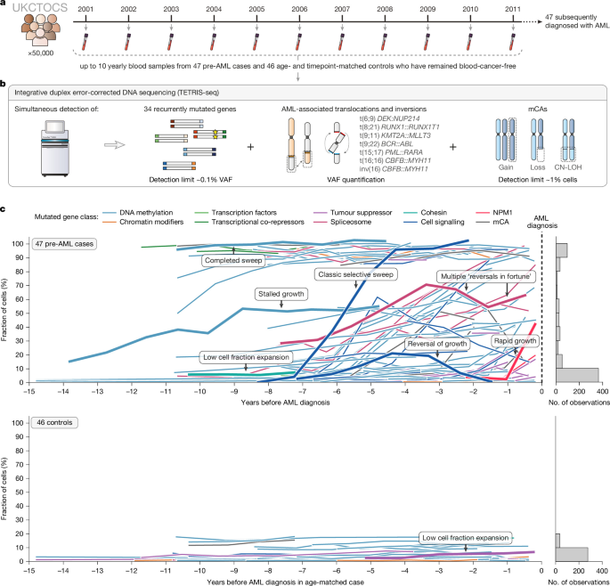
Longitudinal peripheral blood DNA samples
Longitudinal peripheral blood DNA samples were obtained from blood serum samples biobanked as part of UKCTOCS (ISRCTN22488978; ClinicalTrials.gov identifier: NCT00058032). UKCTOCS is a multi-centre randomized controlled trial that recruited 202,638 post-menopausal women aged 50–74 years, from England, Wales and Northern Ireland between 2001 and 2005, to assess the impact of screening on ovarian cancer mortality3. UKCTOCS eligibility criteria and trial details have been described previously58. UKCTOCS was reviewed and approved by the North West Multi-centre Research Ethics Committee (REC reference 00/8/34) and participants provided written, informed consent for use of their samples and data in ethically approved secondary studies. Our study, using UKCTOCS samples and data, was reviewed and approved by the South Central Berkshire B Research Ethics Committee (REC reference 18/SC/0481). This study was performed in accordance with all relevant guidelines and regulations.
At UKCTOCS enrolment, 50,640 participants were randomized to a ‘multimodal screening arm’, which involved annual blood serum samples for up to 11 years, until 31 December 2011. All samples were collected using a standardized protocol. Blood was collected in gel tubes (8-ml gel separation serum tubes; Greiner Bio-One 455071) at the trial centres and transported daily at room temperature to a central laboratory, where the samples were centrifuged (1,500g for 10 min) and the separated serum aliquoted into 10 × 500-µl straws using a semi-automated MAPI platform (IMV). The straws were stored in liquid nitrogen tanks at the central laboratory, which, when full, were transported to an HTA licensed commercial cryofacility (Fisher Bioservices, UK, until March 2018, NIHR Biocentre April 2018 to July 2023 and BioDock since then). The median time from sample collection to centrifugation (about 22.1 h) resulted in leukocyte DNA leaking into the serum59. UKCTOCS participants’ health outcomes were followed via linkage to national cancer, death and administrative registries. By 2017, there were 47 women in the ‘multimodal screening arm’ that had incidentally developed AML (ICD-10 C92.0) and had sufficient serum sample available from at least two timepoints before AML diagnosis. These 47 women were diagnosed with AML at a median age of 72 (range 53–83 years, interquartile range 8 years) and had serum samples biobanked from a median of 5 timepoints (range 2–10, interquartile range 3.5) before AML diagnosis (Extended Data Fig. 1a,b). We obtained 1 ml of serum from each of the yearly timepoints available (249 samples) from these 47 women (‘pre-AML cases’), as well as from timepoint-matched serial samples from 47 age-matched UKCTOCS participants who remained blood cancer free (‘controls’). One control was subsequently excluded owing to development of MDS. No statistical methods were used to predetermine sample size; all eligible pre-AML cases were included. Randomization was not applicable as this was an observational study, and investigators were not blinded to case–control status during sequencing and analysis. DNA was extracted by LGC Genomics, using an adapted Kleargene method with mag beads on KingFisher 96, and eluted in 10 mM Tris-Cl, pH 8.0. The DNA was quantified using PicoGreen, yielding an average of 279 ng ml−1 DNA (range 11–814 ng ml−1 serum) in the pre-AML samples and 270 ng ml−1 DNA (range 11–1,313 ng ml−1 serum) in the control samples (Extended Data Fig. 1c).
Information on any diagnosis of MDS (ICD-10 code D46 or C94.6), CMML (ICD-10 code C93.1) or MPN (ICD-10 codes D45, D47.1, D47.3, D47.4, C92.1, C92.2, C94.4), or other haematological malignancy (for example, lymphoma or myeloma), was obtained for all pre-AML cases and controls via record linkage to the National Cancer Registry (England/Wales), Hospital Episodes Statistics (HES) databases or the Patient Episode Database for Wales (PEDW), the Office for National Statistics mortality records and, for participants in Northern Ireland, the Central Services Agency and Northern Ireland Cancer Registry. Information on diagnoses of non-haematological malignancies was also obtained via linkage to national cancer registries and HES/PEDW databases and Office for National Statistics mortality records. These clinical diagnoses were extracted to characterize antecedent myeloid disease, previous malignancies and treatment exposures that provide clinical context relevant to secondary and therapy-related AML frameworks (see Supplementary Note 5 for detailed case annotations). Where a diagnosis appeared in more than one data source, the earliest recorded entry was taken as the date of diagnosis. Recorded diagnosis dates therefore reflect the first appearance of a diagnosis in national records and may not correspond to biological disease onset. Potential miscoding was assessed by triangulating across available sources: diagnostic entries that appeared only once in HES/PEDW and were discordant with other HES/PEDW episodes, cancer-registry data or death certificate information were treated as probably miscoded and excluded. Information on receipt of chemotherapy (ICD-10 codes Z51.1, Z51.2, Z92.6) or radiotherapy (ICD-10 codes Z51.0, Z92.3) before AML diagnosis (or, for controls, before the matched case’s age at AML diagnosis) was obtained from the HES databases and PEDW. For participants with a record of chemotherapy, the indication was determined by cross-refereeing diagnostic codes in HES/PEDW and/or cancer registry data. Chemotherapy codes temporally associated with AML diagnosis and lacking evidence of a prior malignancy were considered AML-directed and were not classified as pre-AML exposure. No pre-AML case or control was recorded as having received previous radiotherapy. Smoking information, where available, was obtained from UKCTOCS participant questionnaires and HES databases (ICD-10 code Z72.0). The last updates from all linkage sources were received in 2020. As HES and PEDW cover only NHS-funded care in England and Wales, it is possible that diagnoses or treatments delivered privately, abroad or elsewhere in the United Kingdom may not have been captured. Supplementary Table 10 summarizes the timing of any recorded diagnosis of MDS, CMML, MPN or other haematological or non-haematological malignancy, as well as previous chemotherapy exposure and smoking history, for all pre-AML cases and controls, with mortality outcomes (cause of death and survival interval) summarized for pre-AML cases only.
Cell-type deconvolution
To estimate the proportions of different blood cell types (B cells, natural killer cells, CD4+ T cells, CD8+ T cells, monocytes, neutrophils and eosinophils) present in the samples, we used the R package EpiDISH with the reference dataset ‘centDHSbloodDMC.m’60. Whole-genome bisulphite libraries were prepared for 94 UKCTOCS samples from 23 pre-AML cases and 23 controls, some of whom contributed more than one longitudinal timepoint. Of these 94 samples, 88 met the minimum coverage criterion (at least 286 of 333 CpGs covered) and were included in the deconvolution analysis (average depth 7×). Each sample was deconvoluted individually, using the reference CpGs covered in that sample (Supplementary Note 1 and Supplementary Fig. 1).
TETRIS-seq custom panel design
To ensure we could track the evolution of a comprehensive array of clonal haematopoiesis- and AML-associated genomic changes in the longitudinal pre-AML samples and control samples, we developed two separate targeted panels, to be used on the same input DNA sample, in an integrated library preparation approach: a small panel (around 58 kilobases (kb)) specifically for SNVs and indels and a large panel (around 1.6 (megabases (Mb)) for mCA, chromosomal rearrangement and KMT2A partial tandem duplication (KMT2A-PTD) detection (Supplementary Note 2).
For the SNV and indel panel, we designed a custom set of 120-nucleotide (nt) oligonucleotide probes (TWIST Biosciences) targeting commonly mutated exons within 34 genes commonly mutated in clonal haematopoiesis and AML (Supplementary Figs. 2–5 and Supplementary Table 1): ASXL1, BCOR, BCORL1, CBL, CEBPA, CHEK2, CSF3R, DDX41, DNMT3A, EZH2, FLT3, GATA2, GNAS, GNB1, IDH1, IDH2, JAK2, KIT, KRAS, MPL, NPM1, NRAS, PPM1D, PTPN11, RAD21, RUNX1, SF3B1, SRSF2, STAG2, TET2, TP53, U2AF1, WT1 and ZRSR2.
For the mCA, chromosomal rearrangement and KMT2A-PTD panel, we designed a custom set of 120-nt oligonucleotide probes (TWIST Biosciences) targeting a total of 10,326 common SNPs (minor allele frequency > 0.01) spaced every approximately 280 kb across the genome to allow the detection of mCAs (Supplementary Table 2). Using this approach, deviations in heterozygous SNP B-allele frequencies (BAFs) can be detected, which, when combined with read depth information, enable detection of a gain, loss or CN-LOH event. For detection of chromosomal rearrangements, a custom set of 120-nt oligonucleotide baits (TWIST Biosciences) was designed to target the known breakpoint regions of each of the rearranged partner chromosomes61,62,63,64 of seven chromosomal rearrangements that define specific subcategories of AML in the World Health Organization AML classification65: t(6;9) DEK::NUP214, t(8;21) RUNX1::RUNX1T1, t(9;11) KMT2A::MLLT3, t(9;22) BCR::ABL, t(15;17) PML::RARA, t(16;16) CBFB::MYH11 and inv(16) CBFB::MYH11 (Supplementary Fig. 6 and Supplementary Table 3). KMT2A is renowned for having numerous possible breakpoint partners and so further common breakpoint regions in KMT2A were also targeted66. KMT2A-PTDs most commonly involve exon 2 or 3 and span through exons 9 to 11 (ref. 67). They can be detected by observing a relative increase in read depth, starting from exon 2 or 3, compared with an exon that is never involved in KMT3A-PTD (for example, exon 27)68. A custom set of 120-nt oligonucleotide baits (TWIST Biosciences) was therefore designed to target KMT2A exons 2–27 (Supplementary Table 3).
TETRIS-seq error-corrected library preparation and sequencing
TETRIS-seq library preparation was performed as per the ‘TWIST custom panel enrichment workflow’ (TWIST Biosciences), but with adaptations to allow for incorporation of duplex unique molecular identifiers (UMIs), for error-corrected sequencing, and to allow for the use of two targeted panels on the same input DNA. DNA yield varied between UKCTOCS samples (Extended Data Fig. 1), but for each timepoint the same amount of input DNA was used for both the pre-AML sample and matched control (mean 43 ng, median 50 ng, range 4.5–80 ng).
Briefly, DNA was enzymatically fragmented (using the Twist Biosciences proprietary enzyme mix), end-repaired and dA-tailed at 32 °C for 21–24 min (Supplementary Table 4). IDT xGen CS adaptors (5.5 µl of 10 µM), containing 3-bp duplex UMI sequences, were then ligated to each end of the DNA fragments at 20 °C for 15 min, followed by bead purification using 0.8× DNA Purification beads (Twist Biosciences). The duplex UMI-tagged fragments were PCR amplified in a 50-µl reaction volume (25 µl of KAPA HiFi HotStart ReadyMix (Roche Diagnostics), 10 µl of IDT xGen unique dual index primers (10 µM), 15 µl of duplex UMI-tagged fragments). The following conditions were used for PCR amplification: 98 °C for 45 s; 11–12 cycles of 98 °C for 15 s (Supplementary Table 5), 60 °C for 30 s, 72 °C for 30 s; 72 °C for 1 min. Following bead purification, using 1× DNA Purification beads (Twist Biosciences), the amplified UMI-tagged dual index-labelled fragments were eluted into 22 µl of ddH2O and then visualized and quantified using the Agilent 2200 TapeStation.
Following quantification, each sample was divided in two: one half for the SNV/indel panel and the other half for the mCA/chromosomal rearrangement panel. Samples were pooled together in groups of eight (187.5 ng of each indexed sample), with separate pools for each of the two panels. The pooled samples were concentrated, using 1.5× Agencourt AMPure XP beads (Beckman Coulter), and then hybridized to the custom panel probes (SNV/indel panel probes or mCA/chromosomal rearrangement panel probes) in a thermocycler at 95 °C for 5 min followed by 70 °C for 16 h. Following Streptavidin bead capture (30 min at room temperature), the captured DNA was PCR amplified in a 50-µl reaction volume (25 µl of KAPA HiFi HotStart ReadyMix (Roche Diagnostics), 2.5 µl of TWIST amplification primers, 22.5 µl of captured DNA) under the following conditions: 98 °C for 45 s; 12 cycles (mCA/chromosomal rearrangement panel) or 17 cycles (SNV/indel panel) of 98 °C for 15 s, 60 °C for 30 s, 72 °C for 30 s; 72 °C for 1 min. Following bead purification, using 1× DNA purification beads (Twist Biosciences), samples were eluted into 32 µl of ddH2O and then visualized and quantified using the Agilent 2200 TapeStation. Samples were then diluted to 10 nM and submitted for sequencing. Libraries were sequenced on the Illumina NovaSeq 6000 S4 (Cancer Research UK Cambridge Institute Genomics Core Facility) using the XP workflow, with 150-bp paired ends reads, 8-bp reads in index 1 and 8-bp reads in index 2. Forty samples were sequenced per lane, with 10% PhiX control DNA spiked into each lane. SNV/indel and mCA/chromosomal rearrangement panels were sequenced in different lanes and, with only a few exceptions, timepoints from the same individual were sequenced on different lanes. Each sequencing run contained around 3 billion reads per lane (around 68 million reads per sample). For the SNV/indel panel (around 58 kb, 589 probes), this equated to a raw depth (pre-consensus calling) of approximately 50,000×. For the mCA/chromosomal rearrangement panel (around 1.6 Mb, 13,114 probes), this equated to a raw depth of approximately 1,000×.
A custom computational workflow was written for the processing of the sequencing data. This workflow used a number of software packages, including Picard69, Fulcrum Genomics fgio package70, Burrows–Wheeler Aligner (BWA)71, the Genome Analysis Toolkit (GATK)72, SAMtools73, VarDictJava74, Pindel75 and ANNOVAR76, as well as several custom Python scripts. The workflow consisted of four main steps (Supplementary Note 2c): (1) UMI extraction and initial alignment; (2) single strand consensus sequence (SSCS) calling; (3) duplex consensus sequence (DCS) calling; and (4) putative variant detection. For the SNV/indel panel, variants were called from DCS files. The same depth accuracy was not required for the mCA, KMT2A-PTD and chromosomal rearrangement panel and so only the SSCSs were used for these.
TETRIS-seq in silico noise correction model for SNV calling
The theoretical error rate of duplex sequencing is less than 10−9 errors per bp, which is simply the probability of two complementary errors occurring at the same nucleotide position on both DNA strands, either spontaneously or during the first PCR cycle44. In reality, however, library preparation artefacts, for example, due to sonication, end-repair and mapping errors45, have all been shown to slip through the duplex error correction. Therefore, to be able to reliably call variants at ultra-low frequency, we developed an in silico noise correction method for SNV calling (Supplementary Note 2). Our noise correction model is based on the null hypothesis that each base-change at a position in the panel has a specific error rate (\(\varepsilon \)) and the number of variant reads (k) observed in a sample at that position would be consistent with beta-binomial sampling at that specific error rate. A custom Python script was written to infer the error rate (\(\varepsilon \)) and dispersion (\(\delta \)) values for each possible single nucleotide base-change at each position in the panel (hereafter referred to as simply ‘position’) and samples were called as ‘real’ variants if their variant read count was inconsistent with this distribution of errors. First, samples with a VAF > 10% at the position were automatically called as real and excluded from the subsequent analysis. Then, the remaining samples at the position were used to fit a beta-binomial distribution (or a binomial distribution if there were ≤3 samples with ≥1 variant reads). The beta-binomial (or binomial) P values for all the samples with ≥1 variant reads were calculated and a sample was called as a real variant if it’s P value was less than a P value threshold (6 × 10⁻⁶) that gave a false discovery rate of less than 5% (Supplementary Note 2). When fitting a binomial or beta-binomial error distribution to a position only once, a problem arises if more than one sample at the position has a ‘real variant’. The problem is that the lower VAF variants will not be called as they will be fitted as ‘errors’ within a falsely over-dispersed beta-binomial distribution or a binomial distribution with a falsely elevated error rate. We therefore chose to use an iterative approach for positions observed in haematopoietic and lymphoid tissues in COSMIC v.92 (ref. 61) (around 2% of sites across our custom panel), where we might expect to see more than one sample with a real variant in our pre-AML cohort. Similarly, if more than one timepoint sample from the same individual was sequenced on the same sequencing lane, an iterative approach was used for positions at which one of those samples had been called as a real variant. The iterative approach at the position was continued until no further samples from the individual with multi-timepoint samples were called as real. Our in silico noise correction model was applied to all the samples sequenced on the same sequencing lane (around 40 samples) and then further post-processing filters were applied as detailed in Supplementary Note 2g. Somatic variant calls can be found in Supplementary Table 6. On individual trajectory plots, germline variants were annotated where they were rare (absent from ExAC, or with a population allele frequency less than 1%) and not classified as benign or probably benign in ClinVar; genotype (heterozygous or homozygous) was inferred from the mean VAF across timepoints.
TETRIS-seq indels, FLT3 internal tandem duplications and chromosomal rearrangements
Indels were called from DCS files using VarDictJava74 and post-processing filters were applied as detailed in Supplementary Note 2. FLT3 internal tandem duplications (FLT3-ITDs) were identified using Pindel75 and were called as real if detected in both the SSCS and DCS files. A custom chromosomal rearrangement caller was written in Python and validated using serial dilutions of samples with known chromosomal rearrangements (Supplementary Note 2i). The caller used a step-wise algorithm to identify four classes of chromosomal rearrangement. Calling was restricted to the common breakpoint regions of AML-associated rearrangements that were specifically targeted by our sequencing panel (Supplementary Fig. 6). Discordant read pairs and their supplementary alignments were first extracted from these targeted regions to identify candidate breakpoints. Depending on the read configuration, one or both breakpoint partners could be inferred. For discordant reads for which only one partner was identified, soft-clipped regions ≥10 bp were ‘remapped’ by comparing them with breakpoint partner sequences already identified from at least three read pairs; a match was assigned if there was more than 95% sequence match. Concordant soft-clipped reads without discordant alignments were similarly ‘remapped’ by comparing them with breakpoint partner sequences that had been identified by at least five read pairs. VAFs were calculated for each breakpoint as the ratio of supporting reads to local read depth, and the higher of the two breakpoint VAFs was reported. Breakpoint coordinates were annotated using ANNOVAR76 and all calls were subsequently post-processed to refine breakpoint coordinates, remove artifacts and collapse multiple read-based events corresponding to the same underlying rearrangement (Supplementary Note 2i). Chromosomal rearrangement calling was initially performed on the pre-consensus BAM files, but any rearrangements that remained after post-processing were recalled on the SSCS BAM file to enable more accurate VAF quantification.
TETRIS-seq mCA and KMT2A-PTD calling
To detect KMT2A-PTD events, a custom Python script was written (using pysam77 pileup) to calculate the mean read depth across each targeted KMT2A exon. These mean depths were then normalized to the mean read depth across KMT2A exon 27 and the exon 3:27 ratio (R) calculated. The fraction of cells harbouring the KMT2A-PTD is calculated as follows: cell fraction = 2(R − 1) (Supplementary Note 2j).
mCAs were detected from SSCS reads using a custom Python-based caller, developed to exploit both deviations in heterozygous SNP BAFs and read depths (log2R ratios; LRR) in the mCA/chromosomal rearrangement panel, as well as longitudinal haplotype phasing information derived from timepoints at which the same mCA was present at higher cell fraction (Supplementary Note 2k). Loss and gain events result in deviations in both LRR and BAF whereas CN-LOH events result in BAF deviations without a change in LRR (because there is no change in the amount of genetic material) (Supplementary Fig. 25). LRR values were computed from read depths normalized to a panel of normals constructed from 36 control samples, using a leave-one-out strategy for samples within the panel of normals. Five complementary detectors were run independently per chromosome, targeting different signatures of allelic imbalance and copy-number change: a BAF sliding-window detector (run at three window sizes to capture events across a range of sizes), an LRR-first detector, a homozygous-region detector for high cell fraction CN-LOH and loss events, a small-gains detector targeting trisomy-pattern BAF splits and an arm-level detector for subtle whole-arm events. Candidate events were classified as gain, loss or CN-LOH by selecting the event type whose expected LRR best matched the observed LRR, given the BAF-derived cell fraction estimate. Cell fraction was estimated from the heterozygous BAF peak separation using the formulae in Supplementary Table 16. Calls from all five detectors were merged and deduplicated, and CN-LOH events detected at 100% cell fraction at both the earliest and latest available timepoints were classified as likely to be germline and excluded. On the basis of evaluation against an independent simulated test set, which demonstrated substantially reduced sensitivity for events less than 5 Mb, only events greater than or equal to 5 Mb were retained for all downstream analyses (Supplementary Figs. 26–29).
For individuals in whom a somatic mCA was detected, all available longitudinal samples were sequenced and a custom phased longitudinal caller was applied. Haplotype phase was derived from the ‘index sample’, defined as the timepoint closest to AML diagnosis for cases (or the matched timepoint for controls), with the exception of one case (C92_012) in whom the mCA was below the detection of the unphased caller at this timepoint, and so their preceding timepoint was used as the ‘index sample’ instead. Phase was assigned in the ‘index sample’ by comparing each heterozygous SNP’s BAF relative to 0.5. These phase assignments were then applied to all other available timepoints from the same individual, and a one-sided one-sample t-test was used to assess whether the mean phased BAF deviation significantly exceeded zero (P < 0.05). Cell fraction was estimated from the mean phased deviation using event-type-specific formulae (Supplementary Table 16). On simulated test data, the phased caller achieved a 50% sensitivity detection threshold of approximately 1% cell fraction, compared with 20–25% cell fraction for the unphased caller (Supplementary Figs. 26–29). Somatic mCA calls detected in the UKCTOCS pre-AML cases and controls can be found in Supplementary Table 7.
Inferring clonal architecture
A hierarchical step-wise process was used to infer whether a variant was likely to be the only driver mutation in a clone (that is, a ‘single-mutant clone’) or whether it was more likely to be in a clone with one or more of the other variants detected in that individual (Supplementary Table 8). First, we looked at the largest cell fractions for each of the variants detected in an individual: using the pigeon-hole principle, if the sum of the cell fractions for two variants was more than 100% at any timepoint then these two variants were inferred to be in the same clone. Second, we looked at the cell fraction dynamics of the variant trajectories: if the cell fraction trajectories crossed over at any timepoint (that is, one variant’s cell fraction increased to above the cell fraction of another), then these two variants were inferred to be in separate clones. Third, we looked at the correlation in cell fraction dynamics between variants: if the trajectories of two variants showed similar growth dynamics (for example, increasing or decreasing in cell fraction at the same timepoints), then these variants were inferred to be in the same clone. Next, if a larger clone was already present when a new variant was acquired, we inferred that this new variant was more likely to have arisen within the existing larger clone if the larger clone’s cell fraction was more than 50% when the new variant was acquired. Finally, in particular when considering variants that were detected only at timepoints closest to time of AML diagnosis, but that were still present at low cell fraction, we looked at the growth rate of the variant and it’s timing relative to AML diagnosis: the higher the growth rate, and the closer to AML diagnosis the variant was first detected, the more likely we were to infer that the variant was associated with a multiple-mutant clone.
Evolution pattern classification
The evolution pattern for each pre-AML case and control was classified as ‘clonal interference’, ‘late evolution’ or ‘linear evolution’. ‘Clonal interference’ was defined as the presence of multiple driver clones on parallel evolutionary branches, with at least one of these clones expanding to a substantial proportion of the haematopoietic pool (operationally defined as more than 10% cell fraction), thereby influencing the trajectories of other co-existing clones. ‘Late evolution’ was defined as cases in which the putative pre-leukaemic clone was detectable only within 1–2 years before AML diagnosis (or, for controls, before the matched case’s age at AML diagnosis), or where no pathogenic driver mutations (covered by our panel) were detected at all. ‘Linear evolution’ encompassed cases not fitting the above two categories, typically showing sequential acquisition and expansion of driver mutations along a single dominant trunk, with minimal evidence of high-frequency side-branching or competition from parallel high-frequency lineages.
Inferring mutation acquisition age and fitness effect
We developed a mathematical framework for inferring the acquisition age and fitness effects of clones. In this framework each clone (defined by its most recently acquired mutation) has an ‘establishment time’ (\({t}_{0}\)) and fitness effect (s), which determine the clone’s size over time, such that at a particular time (\({t}_{1}\)), the clone size is given by the equation
$${\rm{c}}{\rm{l}}{\rm{o}}{\rm{n}}{\rm{e}}\,{\rm{s}}{\rm{i}}{\rm{z}}{\rm{e}}=\frac{{{\rm{e}}}^{s({t}_{1}-{t}_{0})}-1}{s}$$
(1)
The frequencies of all clones in the population (including non-mutated HSCs) sums to 1, such that at a particular time (\({t}_{1}\)), the clone frequency is given by the equation
$${\rm{c}}{\rm{l}}{\rm{o}}{\rm{n}}{\rm{e}}\,{\rm{f}}{\rm{r}}{\rm{e}}{\rm{q}}{\rm{u}}{\rm{e}}{\rm{n}}{\rm{c}}{\rm{y}}=\frac{{\rm{c}}{\rm{l}}{\rm{o}}{\rm{n}}{\rm{e}}\,{\rm{s}}{\rm{i}}{\rm{z}}{\rm{e}}}{{\rm{s}}{\rm{u}}{\rm{m}}\,{\rm{o}}{\rm{f}}\,{\rm{a}}{\rm{l}}{\rm{l}}\,{\rm{c}}{\rm{l}}{\rm{o}}{\rm{n}}{\rm{e}}\,{\rm{s}}{\rm{i}}{\rm{z}}{\rm{e}}{\rm{s}}\,{\rm{i}}{\rm{n}}{\rm{c}}{\rm{l}}{\rm{u}}{\rm{d}}{\rm{i}}{\rm{n}}{\rm{g}}\,{\rm{w}}{\rm{i}}{\rm{l}}{\rm{d}}\,{\rm{t}}{\rm{y}}{\rm{p}}{\rm{e}}}$$
(2)
The dynamics of a specific variant, directly measured via the variant’s VAF, are determined by summing the frequency of the original parental clone (that is, the first clone to acquire the variant) and all daughter clones that inherited the variant. Using this framework, together with inferences for the clonal architecture of each sample (as described above), we developed a maximum likelihood approach to infer fitness and establishment time estimates for each clone in the population by comparing the predicted VAF trajectories with the observed VAF trajectories in all pre-AML cases and controls. To assign a likelihood to the observed data, given the predicted trajectories, we developed a likelihood function as follows: for each variant at each timepoint, we assigned a likelihood to the observed number of variant reads using a binomial probability with mean given by the predicted frequency and sample size given by the total depth at that position in the sample. The log(likelihoods) were summed across all the variant timepoints for all trajectories and our maximum likelihood approach minimized the sum of all the total log(likelihoods).
Our maximum likelihood optimization approach started with an ‘initial estimate’ for the establishment time and fitness of each clone. Depending on the number of VAF timepoints, this was typically estimated from the gradient of a straight line drawn through the log(VAF) trajectory (with or without ‘bounded VAFs’ for undetectable VAF timepoints) or was on the basis of the number of mutations in the clone (Supplementary Note 4). Once the ‘initial estimate’ for the establishment time and fitness of each clone had been set, a three-stage maximum likelihood process was applied. Within each stage, approximately 1,000–5,000 optimizations were performed, with adjustment of the establishment time and fitness with each optimization to find the lowest total log(likelihood) across all trajectories in that sample. Each of the three stages involved progressively finer adjustments in the predicted establishment time and fitness of the clone with each optimization (similar to simulated annealing). Penalties were applied to the log(likelihoods) in certain situations, for example, to account for timepoints at which a variant was undetectable (Supplementary Note 4). For each sample, the three-stage maximum likelihood process was repeated for 25 ‘seeds’ and the results of the seed that produced the lowest total log(likelihood) were taken as the most likely establishment times and fitnesses for the variants in that sample.
To quantify the uncertainty around our fitness and establishment time estimates, we considered all ‘seeds’ whose likelihood scores were within ±20% of the best (lowest) log(likelihood). From these, we calculated two measures of uncertainty: (1) the 95% range of the parameter estimates across these seeds (‘95% optimizer range’), defined as the central interval containing 95% of the values, and (2) the standard deviation of these parameter values (Supplementary Note 4, Supplementary Fig. 46 and Supplementary Table 9).
A simulated model of evolutionary dynamics in blood
In this model, blood is maintained by a population of N cycling HSCs that divide symmetrically every \(\tau \) years, modelled as a continuous-time, birth-death process39. Asymmetric divisions can occur in this framework, but they do not affect clone sizes and therefore are not explicitly modelled. HSCs acquire driver mutations at a rate U per year. Driver mutations vary in the fitness effects they confer to HSCs. The fitness effects are drawn from a probability density distribution that is modelled using a stretched exponential as described previously40:
$$\rho (s)=\frac{1}{{\mathscr{N}}}\exp \left(-{\left(\frac{s}{{r}^{k-1}{s}_{0}}\right)}^{p}\right)$$
(3)
where \({\mathscr{N}}\) is a normalization constant and k is the number of driver mutations in the clone, and where we have set p = 3, r = 2.5. A driver mutation arising in a wild-type HSC, creating a single-mutant clone, confers fitness advantages drawn from a distribution with a median and range controlled by a single parameter \({s}_{0}\) = 16% per year. A driver mutation arising in a single-mutant clone confers a median fitness effect that is r = 2.5-fold larger (typical fitness effects s = 40% per year), creating a double-mutant clone. Triple- and quadruple-mutant clones follow the same geometric pattern (with median fitness effects of s ≈ 100% and s ≈ 250% per year, respectively). Fitness advantages of driver mutations combine additively in this model, such that the growth rate of a clone carrying k driver mutations is given by
$$\Delta =\mathop{\sum }\limits_{i}^{k}{s}_{i}-\bar{x}$$
(4)
where \(\bar{x}\) is the mean fitness of all clones in the population weighted by their clone size and where \({s}_{i}\) represents the fitness advantages of each of the driver mutations in the clone. Transformation to frank AML is defined by the acquisition of four driver mutations within the same clone that reaches more than 50% cell fraction before the age of 85. Using established estimates of \(N\tau \) = 105, U ≈ 10−5 per year and s ≈ 16% per year for single-mutant fitness effects, we simulated clonal dynamics in 200,200 simulations and considered the evolutionary dynamics observed in the decades preceding the 943 virtual incidental AMLs.
High VAF variants in the UK Biobank
Clonal haematopoiesis variants were called in UK Biobank participants with exome sequencing data. Individuals with a history of cancer before the UK Biobank baseline assessment (including self-reported cancer, excluding basal cell carcinoma, pre-cancer of the cervix and rodent ulcer) were excluded, leaving 424,089 individuals. Individuals who developed other haematological malignancies after baseline were also excluded (n = 4,035), leaving 420,054 individuals for analysis. The North West Multi-centre Research Ethics Committee reviewed and approved the UK Biobank scientific protocol and operational procedures (REC 21/NW/0157) and all participants provided signed, informed consent at enrolment. Variants were called at 27 genomic positions previously identified as the locations of clonal haematopoiesis driver variants39 from the UK Biobank exome CRAM files using samtools mpileup on the DNANexus Research Analysis Platform (UK Biobank Application Number 58387): DNMT3A R320*, R326C/G/S, R598*, R729G/W, Y735C/F, R736C/G/H/L/S, R771*, R882H/C/S/L/P, W860R, P904L/Q/R; GNB1 K57E; IDH1 R132H; IDH2 R140Q, R172K; JAK2 V617F; KIT D816F/H/V/Y; KRAS G12C/D/V; MPL W515L; NRAS G12C/D/V; SF3B1 K666N, K700E; SRSF2 P95H/L/R. Variants with less than three supporting reads were discarded. A total of 516 individuals were identified who were diagnosed with myeloid leukaemia (ICD-10 C92) after the UK Biobank baseline assessment (‘prospective cases’). In total, 5,034 individuals carried at least one of the clonal haematopoiesis variants analysed, of whom 114 represented prospective cases. A total of 106 individuals carried two clonal haematopoiesis driver variants, of whom 23 represented prospective cases. Somatic sweeps were defined as at least one variant at VAF > 30%; 388 individuals had a somatic sweep, of whom 42 represented prospective cases. Associations with prospective myeloid leukaemia were assessed using a two-sided Fisher’s exact test against all other participants.
Statistics and reproducibility
No statistical methods were used to predetermine sample size: all individuals in the ‘multimodal arm’ of UKCTOCS who had been diagnosed with AML by 2017, and who had sufficient serum sample available from at least two timepoints before AML diagnosis, were included.
Reporting summary
Further information on research design is available in the Nature Portfolio Reporting Summary linked to this article.