
Methodology
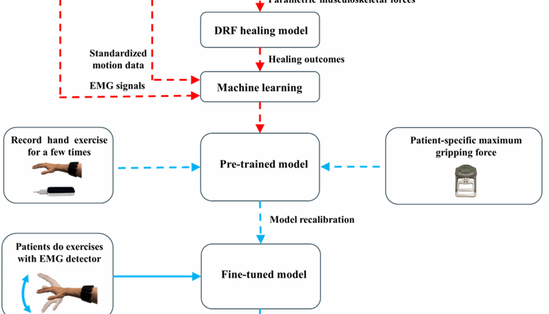
The methodology of this study is illustrated in Fig. 1, which includes collecting data from volunteers, processing the data using well-validated musculoskeletal and DRF models to conduct a parametric study, developing a machine learning model, recalibrating the model based on patient-specific data, and delivering biofeedback when predicted healing outcomes fall below a defined threshold. The following sections provide a detailed explanation of each component.
Fig. 1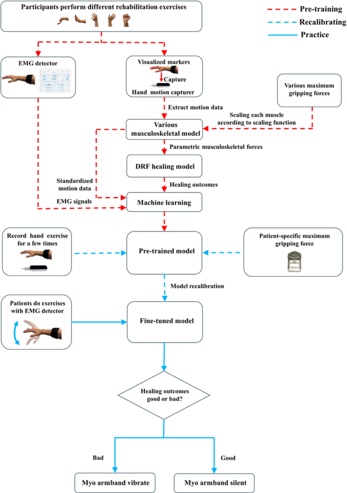
Methodology path of this study
Data collection
In the initial stage of data collection, 67 healthy volunteers without injuries or chronic conditions were recruited. The initial dataset had a higher proportion of young and male participants. To ensure demographic balance, a random selection process was applied to achieve equal representation of males and females, and to stratify age groups in 5-year increments from 18 to 65 years. As a result, 20 volunteers (10 males and 10 females) were selected. The mean age of the selected group was 41.3 years. This approach ensured diversity across both age and gender, supporting model generalisability. The selection strategy was designed to minimise potential bias, enhance the database’s inclusiveness, and improve the model’s robustness and generalisability across different populations.
Figure 2 shows the equipment setup and their relative positions during data collection. The setup included a Leap Motion Controller for capturing hand motion and a Myo armband for recording EMG signals. The two devices were positioned approximately 30 to 60 cm apart to ensure optimal hand tracking within a 120 × 150° field of view. Both devices were operated by the same processor to maintain data synchronisation.
Fig. 2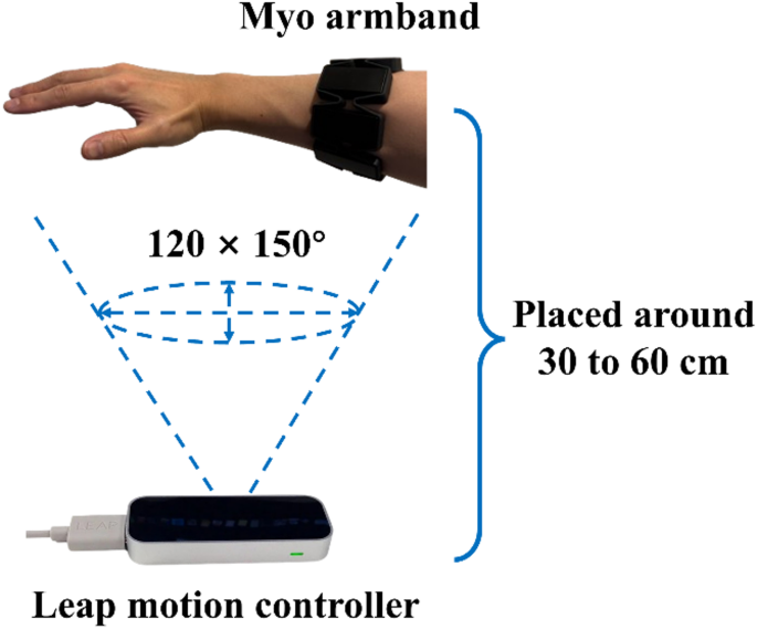
Sketch of Leap motion controller and Myo armband parallel positions during data collection
Hand motion data
The Leap Motion Controller is a depth camera specifically designed for hand motion tracking. Its accuracy has been validated in previous studies for motion tracking [19, 20, 21]. Although it does not match the precision of high-end marker-based systems such as Vicon, it provides a practical and cost-effective alternative for real-world applications. Unlike marker-based systems, which require specialised hardware, designated laboratory space and trained personnel, the Leap Motion Controller is lightweight, portable and does not require physical markers. These features make it particularly well suited for use in both clinical and home-based rehabilitation settings.
As shown in Fig. 3(a), 23 visualised marker positions were extracted using the Leap Motion Controller’s software development kit, including markers on the forearm, wrist, palm, and finger joints, to reconstruct detailed hand motions. This setup ensures reliable motion tracking while maintaining practicality and accessibility in rehabilitation scenarios.
At the initial stage of data collection, volunteers watched an instructional video explaining the exercises they were required to perform, including relaxation, flexion/extension, radial/ulnar deviation, and fisting. During the relaxation phase, volunteers placed one hand over the Leap Motion Controller, maintaining a 30 to 60 cm distance, and remained as relaxed as possible. For the subsequent exercises, including flexion/extension, radial/ulnar deviation, and fisting, the volunteers were instructed to move gently through their maximum range of motion while maintaining an approximate exercise rate of 1 Hz, as recommended by Liu et al. [22]. The volunteers were asked to perform the exercises gently to mimic the limited movement capacity of patients with DRFs, where excessive force or speed may lead to secondary injury. Moreover, controlled movements help reduce signal fluctuations, ensuring smoother and higher-quality data for machine learning training. The exercises were performed in sequence, with each lasting 2.5 s. To prevent muscle fatigue, a short pause was included between exercise types, allowing volunteers to rest. After smoothing and removing background noise using MATLAB 2023b, the motion data were saved as .csv files with system timestamps to synchronise with EMG signals.
EMG data
Traditional EMG collectors are usually restricted to laboratory settings and require multiple electrodes to be manually setup by researchers. While Myo armband is an integrated device, which is portable and convenient. It consists of eight channel electrodes arranged in a circular configuration to capture the wearer’s muscle electrical signals. Myo armband is worn around the forearm for use. It is suitable for both clinical and everyday applications. The instructional video provided a demonstration on how to correctly and uniformly wear Myo armband, as shown in Fig. 3(b). Electrode 1 was aligned with the wearer’s middle finger to ensure consistency in data collection and improve the comparability of recorded signals. Electrodes 1 through 4 monitored flexor muscle activations, electrodes 5 and 6 recorded extensor muscle activation, and electrodes 7 and 8 captured mobile wad muscle activation.
Volunteers wore the Myo armband while performing exercises to record EMG signals. Signals from all eight channels were recorded using the Myo armband’s software development kit. However, the raw EMG signals contained significant noise and required preprocessing before use. To preserve essential signal characteristics while minimising noise, the EMG signals were processed in two steps. First, they were pre-processed using a band-pass filter with rectification at 50 Hz. This step attenuated power line interference and isolated relevant muscle activity signals. Next, a moving average smoothing function with a window size of five was applied to further reduce noise and enhance signal continuity while preserving the overall signal integrity.
Since the Myo armband records at 50 Hz and the Leap Motion Controller records at 60 Hz, a mismatch in sampling rates existed between the two data sources. Additionally, some data loss occurred during signal collection. To address these issues and improve system consistency, the sampling frequency was standardised to 30 Hz. To achieve this, timestamps were added during both motion and EMG data collection. Specifically, the motion data were resampled to 30 Hz by averaging every two consecutive data points and aligning them with the nearest EMG signal timestamp. Although the original sampling rates differed, the time gap between synchronised data points remained under 7 milliseconds, ensuring precise alignment without significant mismatch. Following this processing, the hand motion and EMG signal datasets were synchronised, allowing for accurate and reliable subsequent analysis.
Fig. 3
(a) Visualized markers captured by Leap motion controller and (b) proper placement of Myo armband
Musculoskeletal model
Figure 4 demonstrates the applied musculoskeletal model [23], which is referred to as the standard model in the following paragraphs. It is based on the open-source software OpenSim 4.4. The model includes 45 active muscles, whose force-length characteristics are described by the ‘Millard2012EquilibriumMuscle’ model [24]. Additional key muscle properties, including physiological cross-sectional area, peak isometric forces, optimal fibre lengths, pennation angles, and slack lengths, were sourced from McFarland et al. [23]. The model consists of 24 degrees of freedom, which allows for complex forearm motions such as pronation and supination, wrist movements including flexion, extension, radial deviation, and ulnar deviation, as well as finger joint motions such as abduction and flexion. Additionally, ligament effects during movement are incorporated into the model using position-dependent torques described by Eq. 1 [16]. Detailed torque parameters are provided in Table 1, which are sourced from Li et al. [18]. These configurations ensure a highly detailed and realistic simulation of hand and forearm dynamics.
$$\:\begin{array}{c}{\tau\:}_{i}=\frac{{\tau\:}_{max,i}\cdot\:{\theta\:}^{n}}{{K}^{n}+{\theta\:}^{n}}\end{array}$$
(1)
where \(\:{\tau\:}_{i}\) is the torque on the wrist under different motion types i, \(\:{\tau\:}_{max,i}\) is the maximum torque, \(\:\theta\:\) is the degree of motion range, \(\:K\) is the apparent constant, and \(\:n\) is the Hill coefficient.
Table 1 Parameters of position-dependent torques at different motions [18]Fig. 4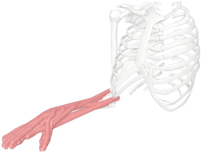
Sketch of the musculoskeletal model applied in this study
Furthermore, individual muscle strength plays a critical role in accurately simulating musculoskeletal forces, which in turn significantly influences the prediction of healing outcomes. Li et al. [25] proposed a scaling function that incorporates individual muscle strength by adjusting the standard musculoskeletal model. Specifically, they derived a fitting curve based on the dataset from Wind et al. [26], which demonstrated a strong linear relationship between grip force and overall muscle strength. They also calculated the grip strength of the standard musculoskeletal model to be approximately 250 N. Using this information and the derived curve, a scaling function was extracted (see Eq. 2). Simulation results based on the scaling function aligned closely with experimental measurements, validating its effectiveness in personalising musculoskeletal models. By adjusting the maximum isometric force of each muscle according to an individual’s measured or targeted grip strength, the function enabled the generation of personalised models.
Accordingly, in this study, the standard model was scaled to produce 20 distinct versions, each representing a grip force ranging from 100 N to 500 N in evenly spaced increments. Each volunteer’s hand motion data was then integrated into these 20 musculoskeletal models to perform parametric simulations for subsequent FEM-based modelling. This process aimed to establish a comprehensive benchmark for machine learning model training. In terms of workflow, hand movements were reconstructed using the inverse kinematics approach, muscle forces were estimated via the static optimisation method, and bone-to-bone contact forces were calculated using the joint analysis function. Further details are available in Li et al. [27]. Additionally, each volunteer’s maximum grip strength was measured using a digital dynamometer to provide a personalised reference for selecting the most representative model output among the 20 simulated variants. For example, a subject with a measured grip strength of 265 N would be matched to the musculoskeletal model corresponding to 260 N. This process balanced inter-individual variability in muscle strength with the computational cost of subsequent FEM-based simulations.
$$\:\begin{array}{c}C=\frac{{F}_{m}}{{F}_{m,standard}}=\frac{{F}_{g}+81.55}{328.23}\:({F}_{g}>0)\end{array}$$
(2)
where \(\:C\) is the scaling coefficient, \(\:{F}_{m,\:\:standard}\) is the muscle strength (N) of the standard model, \(\:{F}_{m}\) is global muscle strength (N), and \(\:{F}_{g}\) is maximum grip force (N).
DRF healing model
The simulated musculoskeletal forces were input into our well-developed FEM-based DRF model [15, 16, 22]. To manage computational cost, the simulation was configured to represent the early healing stage (week 3), with a fracture gap size of 1 mm. As shown in Fig. 5, this DRF model includes realistic bone geometry and VLP fixation. The model geometry was reconstructed from computed tomography scan images using SolidWorks (Dassault Systèmes, MA, USA). The dimensions of the VLP were provided by Austofix (SA, Australia). The VLP models were symmetrised for numerical simulation using COMSOL Multiphysics 6.0 (COMSOL Inc., MA, USA). Detailed mechanical properties of the bone and VLP components are provided in Table 2 and further described in the work of Liu et al. [15].
Fig. 5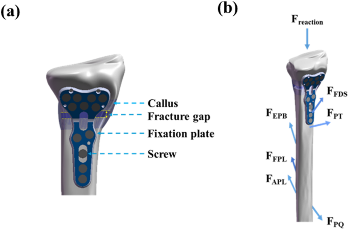
Sketch of distal radius fracture (DRF) model (a) its structures and (b) applied reaction force and muscle forces, including Abductor Pollicis Longus (APL), Extensor Pollicis Brevis (EPB), Flexor Digitorum Superficialis (FDS), Flexor Pollicis Longus (FPL), Pronator Quadratus (PQ), and Pronator Teres (PT) muscles
Table 2 Material properties used in the DRF healing model [15]
$$\:\begin{array}{c}S=\frac{{\tau\:}^{s}}{a}+\frac{{v}^{f}}{b}\end{array}$$
(3)
where \(\:{\tau\:}^{s}\) is the octahedral shear strain of solid tissues, \(\:{v}^{f}\) is the flow velocity of the interstitial fluid, a is constant (a = 0.0375), and b is standard flow velocity (b = 3\(\:\mu\:m/s\)).
The model accounts for reaction forces (bone-to-bone contact forces) and muscle forces acting directly on the radius. It includes the Abductor Pollicis Longus (APL), Extensor Pollicis Brevis (EPB), Flexor Digitorum Superficialis (FDS), Flexor Pollicis Longus (FPL), Pronator Quadratus (PQ), and Pronator Teres (PT) muscles. When mechanical stimuli are low (S-index < 1), MSCs are induced to undergo intramembranous ossification, forming compact nodules that eventually develop into bone tissue. For moderate levels of mechanical stimuli (1 < S-index < 3), the increased stress induces MSCs to differentiate into chondrocytes, promoting the formation of cartilage tissue and facilitating endochondral ossification. When the S-index exceeds 3, it indicates excessive biomechanical loading, which leads to the formation of fibroblasts and fibrous connective tissue, resulting in delayed healing or non-union of the fracture.
The model applied porous media theory to simulate the local mechanical micro-environment of the callus, effectively capturing deformation and fluid flow within its porous structure. The governing equations for porous media theory are presented as follows [28]:
$$\:\begin{array}{c}\sigma\:=-pI+{\varvec{\sigma\:}}^{\varvec{e}}\end{array}$$
(4)
$$\:\begin{array}{c}{\varvec{\sigma\:}}^{\varvec{e}}=\frac{1}{{J}^{s}}{\varvec{F}}^{\varvec{s}}\cdot\:2\frac{\partial\:\left({W}^{s}\right)}{\partial\:{\varvec{C}}^{\varvec{s}}}\cdot\:{\varvec{F}}^{{\varvec{s}}^{\varvec{T}}}\end{array}$$
(5)
$$\:\begin{array}{c}\nabla\:\cdot\:\sigma\:=-\nabla\:p+\nabla\:\cdot\:{\varvec{\sigma\:}}^{\varvec{e}}=0\end{array}$$
(6)
$$\:\begin{array}{c}\nabla\:\cdot\:\left({\varvec{v}}^{\varvec{s}}-\text{K}\nabla\:p\right)=0\end{array}$$
(7)
where \(\:\varvec{\sigma\:}\) is the stress tensor of tissues, \(\:p\) is the interstitial fluid pressure, \(\:\mathbf{I}\) is the identity matrix, \(\:{\varvec{v}}^{\varvec{s}}\) is the velocity of the solid phase, \(\:\text{K}\) is the permeability tensor of tissues, \(\:{\varvec{\sigma\:}}^{\varvec{e}}\) is the effective stress, \(\:{\varvec{F}}^{\varvec{s}}\) is the deformation gradient, \(\:{W}^{s}\) is the strain energy density, \(\:{\varvec{C}}^{\varvec{s}}\) is the right Cauchy-Green deformation tensor, and \(\:{J}^{s}\) is the volume change of the solid matrix, respectively.
Machine learning
FEM-based simulations are time-consuming, and their duration depends on the length of the rehabilitation exercises being modelled. For example, simulating 10 s of real-world exercise requires approximately one week of computation. Thus, the FEM-based healing model is impractical for direct real-time biofeedback applications. To overcome this computational challenge, this study incorporated machine learning to accelerate the simulation process. It aims to directly predict fracture healing outcomes from EMG signals and deliver real-time biofeedback to users when the estimated outcomes fall below a predefined clinical threshold.
However, during preprocessing data, it was found that individuals exhibited distinct EMG signal patterns for the same motion type, despite careful alignment of the wearable device. Moreover, volunteers deviated from idealized hand motions. For example, during flexion/extension exercises, many volunteers unintentionally introduced varying degrees of deviation and fisting. Given such varieties in EMG patterns and hand motions, as well as the difference in individual muscle strength, using only EMG signals is insufficient to reliably predict rehabilitation outcomes through machine learning. To improve data relevance and reduce noise, the 23 hand marker positions were standardized using inverse kinematics with the musculoskeletal model. This enabled the characterization of hand motions using three principal components: flexion/extension, radial deviation, and fisting (represented by middle finger flexion). They were normalised with respect to their range of motion, scaled from 0 to 1, and grouped according to motion types. For example, flexion and extension were treated as a pair, forming a set ranging from − 1 to 1, as they represent opposing directions of movement. After preprocessing, each volunteer’s dataset contained information captured from 10-second exercises, sampling at 30 Hz, and the maximum gripping force from muscle strength assessment. Features are listed below:
Eight channel EMG signals from the Myo armband.
Three principal normalized components, flexion/extension, radial deviation, and fisting, representing hand motions in exercises.
Individual maximum gripping force.
Parametric simulation results of tissue compositions (bone, cartilage, fibrous tissue; total of 1.0) from a validated FEM-based DRF model.
As shown in Fig. 6, a systematic framework was implemented to strengthen and capture the relationship between EMG signals and individualised fracture healing outcomes. It includes three sequential machine learning steps (models). In Step 1, the model learns the mapping from eight-channel EMG signals to the three principal components of hand motion: flexion/extension, radial deviation, and fisting. In this step, the standardised set of 23 hand marker positions was used as ground truth to evaluate model performance. The model was also fine-tuned using user-specific EMG signals and each user’s maximum grip strength to improve accuracy and adaptability for personalised rehabilitation in real-world clinical applications. In Step 2, the predicted hand motion components and individual maximum grip strength were combined to estimate tissue-level healing outcomes. The maximum grip strength was used as a key reference to match each input with the most representative case from the set of parametric simulations. The target outputs were obtained from the FE-based DRF healing model under the corresponding representative condition. In Step 3, the models from Step 1 and Step 2 were integrated into a unified pipeline, enabling direct prediction of healing outcomes from EMG signals and maximum grip strength.
Fig. 6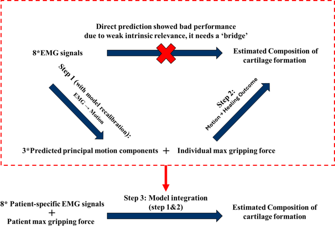
Training pipeline of the machine learning model development, which includes three steps; Step 1 EMG to motion prediction; Step 2 motion to healing outcome; Step 3 EMG to healing outcome with model recalibration
Several machine learning approaches were selected and evaluated. Considering the non-linear relationships between EMG signals, hand motions, and simulated healing outcomes, Random Forest (RF) and K-Nearest Neighbour (KNN) were chosen for evaluation. In addition, as the collected data are sequential, Recurrent Neural Network (RNN), Convolutional Neural Network (CNN), and Long Short-Term Memory (LSTM) networks were also considered.
During training, cross-validation was employed to mitigate bias and overfitting while enhancing model reliability and robustness. To optimize model performance, each model used cross validation in three folds and underwent structured hyperparameter tuning. For RF, grid search was conducted over the number of estimators (50, 100, 200), maximum tree depth (5, 10, 20), and minimum samples per split (0.01–0.1). The KNN model was optimized by selecting the number of neighbours (1–20) that minimized root mean square error (RMSE). For deep learning models, key parameters including number of layers (1–3), hidden units per layer (32–128), learning rate (1e-4–1e-2), batch size (16–64), and activation function (ReLU, tanh) were tuned. Dropout rates (0.1–0.5) and optimizers (Adam, RMSprop) were also considered. Early stopping criteria were applied to prevent overfitting, and model convergence was monitored via validation loss curves.
The step 1 model was also recalibrated with patient-specific EMG data via training new trees (for RF); appending new data to existing dataset (for KNN); proceeding transfer learning (for deep learning models) in step 3 to better predict hand motions. The model performance was tested using four independent testing datasets and evaluated by multiple metrics, including coefficient of determination (R²), root mean square error (RMSE), paired t-test p-value against ground truth, and Cohen’s d effect size. A detailed analysis and discussion of all statistical results can be found in ‘3.4. Statistical Analysis of Model Performance’.
Trial case
To evaluate the model’s real-world applicability, a trial case was conducted using one of the four independent testing datasets, representing a simulated patient. As described in previous sections, the most representative musculoskeletal model was selected based on the individual’s maximum grip strength. Musculoskeletal forces were computed and input into the DRF healing model to generate simulated healing outcomes. At the same time, the pre-trained machine learning model was fine-tuned using the volunteer’s EMG data. The personalised, fine-tuned model was then used to predict healing outcomes, which were subsequently compared with the FEM-based simulation results. This comparison aimed to validate the accuracy and reliability of the machine learning model within a realistic clinical scenario.