Mobile phone data show spatial and socioeconomic inequalities in hospital utilization

Data

This study utilized mobile phone Global Positioning System (GPS) data provided by Moxing Beijing from 1 April to 31 May 2023 in 11 sampled cities of China. The location collection mechanism resembles the widely used SafeGraph dataset in the USA, primarily comprising de-identified GPS location pings from smartphones. The data gathered via smartphone applications with users’ explicit consent guarantees anonymity and adherence to privacy regulations, free from any linkage to personally identifiable information such as names, phone numbers or email addresses. The data’s representativeness was validated (Supplementary Fig. 2), although it may not fully represent individuals who decline location sharing or use mobile phones infrequently. The raw dataset consists of 96,008,397 users, with an average of 30 pings per user per day. Each ping is composed of a de-identified ID, longitude, latitude and timestamp.

Hospital areas of interest (AOIs) were obtained from Baidu Maps, China’s largest map service provider. In addition, 65 hospitals were marked as prestigious based on the authoritative Fudan Chinese Hospital League Table (Fudan CHLT) ranking system34. To estimate patients’ SES, we gather the average property value (CNY m−2) of patients’ home location, which provides more accurate SES measurements than income survey in aggregated level19. Then, we classified the patients into high (top 20%), middle (20–80%) and low-SES groups (last 20%) based on their property value within a city. Residence house price data were collected from Lianjia and Anjuke, two major Chinese real estate information platforms. Road network data were sourced from OpenStreetMap.

Hospital visits identification

We first detected potential hospital visits by identifying spatial intersections between users’ trajectories and hospital AOIs. A record was classified as a potential hospital visit if a user’s trajectory intersected with a hospital AOI and the dwelling time within the AOI exceeded 30 min (ref. 35). This threshold helps to distinguish substantive hospital visits from brief pass-through events (for example, people walking near or through hospital grounds without seeking care). Subsequently, we applied filtering rules based on visit duration and visit frequency to exclude hospital staff. Users appearing in the same hospital AOI on more than one-third of days within the 2-month study period were classified as hospital staff rather than patients because both outpatients and inpatients have much lower visit frequencies. Typical outpatient treatments involve one or a few visits within a short period, whereas inpatients do not exhibit the daily in-and-out hospital AOI mobility patterns characteristic of hospital staff. This conservative criterion excludes most non-patient users while minimizing the risk of mistakenly removing long-stay patients. Finally, we excluded the potential accompanying family members using trajectory-based contact detection and graph-theoretic network analysis (see details in ‘Accompanying family members identification’ section).

We identified a total of 8,052,033 hospital visits made by 6,451,053 unique hospital patients after applying the spatiotemporal filtering and exclusion criteria. Among identified hospital visits, the duration distribution shows that most visits are relatively brief, consistent with outpatient care patterns (Supplementary Fig. 14). The concentration of visits in the 1–3 h range (61.6% combined) is consistent with typical outpatient processes in Chinese hospitals. The smaller proportion of extended-duration visits (>5 h, totalling approximately 24%) probably represents patients requiring extended observation (for example, diagnostic tests).

Sensitivity analysis

We conducted comprehensive sensitivity analyses to assess the stability of hospital visit identification across alternative threshold specifications, including visit durations of 30, 45 and 60 min, and visit frequencies of 15, 20 and 30 days. We examined all nine combinations of these thresholds and their impacts to our major finding (Supplementary Table 6 and Supplementary Fig. 11). All key findings including bypass prevalence, bypass cost and bypass SES disparities remain robust. These results confirm that our findings are not artefacts of arbitrary threshold choices but reflect genuine behavioural patterns in hospital utilization.

Hospital visit validations

We validated our patient identification against three independent metrics from the China Health Statistical Yearbook and local hospitals reports. (1) We classified patients as hospitalized if their trajectories showed continuous dwelling within a hospital AOI for ≥3 consecutive days, distinguishing inpatient stays from outpatient visits (after excluding hospital staff). Applying this criterion to our 2-month dataset, we calculated hospitalized patients with an estimated 4.25% hospitalization rate. The difference between our estimate and the official national statistic (4.2%) is 0.05%. (2) During the 2-month observation period (April to May 2023), the distribution of visit frequencies shows that 55.3% of identified patients made only one hospital visit, and the ratio of total visits to unique patients is 1.25 visits per patient. We calculated the implied annual visit frequency by multiplying the observed average (1.25 visits per patient over 2 months) by 6, yielding an estimated 7.5 visits per person per year, which is close to the official national statistic (6.78 hospital visits per person). (3) We compared our identified hospital visit volumes against local hospital report that only available in Shenzhen City, which show strong correlation R2 = 0.91, P < 0.001 (Supplementary Fig. 2).

Accompanying family members identification

We developed a comprehensive two-stage approach combining trajectory-based contact detection19 with graph-theoretic network analysis to identify patient–companion relationships. We define a ‘contact’ between two individuals as occurring when their coordinates are within a specified spatial distance threshold (50 m) for a specified temporal duration (30 min). We require contacts to occur in three distinct locations—residence, hospital and transit—to establish a patient–companion relationship.

To distinguish patient from companions, we construct an undirected graph G = (V, E) for each city, where each individual is a node and each identified contact relationship is an edge. Our core assumption is that patients typically serve as ‘hubs’ connecting one or multiple companions, which can be identified from network metrics including global and local clustering coefficient, network density and degree distribution. Based on these metrics, we classify connected components into four structural types and identify both patient and companion (Supplementary Table 3).

The estimated accompanying rates for all 11 cities are consistently low. We conducted sensitivity analyses using nine combinations of spatial and temporal thresholds for contact definition including: spatial thresholds of 30 m, 50 m and 80 m, and temporal thresholds of 15 min, 30 min and 45 min (Supplementary Tables 4 and 5). All main text results reflect the analysis after excluding identified companions using the 50-m and 30-min threshold.

NNHI

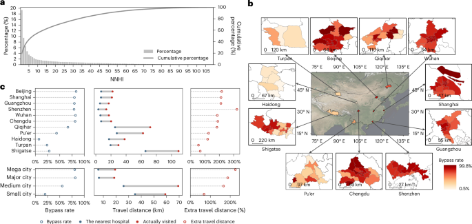
The NNHI was introduced to depict patients’ hospital bypass behaviours. NNHI is computed by sorting the road network distances between patients’ residences and all city hospitals in ascending order and identifying the rank of the actual visited hospital. This rank represents the NNHI value, reflecting patients’ willingness to prioritize more distant hospitals over closer ones. For example, an NNHI of 5 indicates visiting the 5th nearest hospital (bypass behaviour), while an NNHI of 1 suggests visiting the closest hospital (non-bypass behaviour).

IV analysis to isolate exogenous variation in SES

To isolate exogenous variation (for example, disease severity) in SES analysis, an IV approach is applied36. IV analysis uses a variable (the instrument) that is strongly correlated with the exposure of interest (SES), but plausibly unrelated to the unobserved confounders that directly influence the outcome (for example, disease severity), which can recover the component of SES variation that is exogenous (that is, not driven by health status or medical demand). We use school district as instruments for residential property value (our SES measure)37. Proximity to a high-quality school strongly influences housing prices (relevance) but should not directly affect clinical need (exclusion restriction). Therefore, school proximity affects bypass behaviour only through SES.

SEM for decomposing SES mechanisms

SEM was built to explore through which pathways SES operates bypass behaviour. It estimates direct effects of SES on bypass behaviour, as well as indirect effects operating through multiple mediating mechanisms, and tests whether the SES and bypass relationship persists when accounting for complex causal pathways that could otherwise confound traditional regression estimates38. Home–hospital distance, hospital reputation and tertiary hospital ratio (concentration of tertiary grade A hospitals in the area) are considered as mediating structural factors. These mediators represent spatial and institutional features of the healthcare system rather than individual patient attributes, which test whether SES effects operate through the healthcare environment structure.

Hospital accessibility

Hospital accessibility was evaluated using the E2SFCA method39. Hospital accessibility (\({{{A}}}_{{{i}}}\)) at demand point i is calculated as

$${{{A}}}_{{{i}}}=\sum _{{{j}}\in {{{t}}}_{{{ij}}}\le {{{T}}}_{{{r}}}}{{{R}}}_{{{j}}}{{{W}}}_{{{r}}}=\sum _{{{j}}\in {{{t}}}_{{{ij}}}\le {{{T}}}_{{{r}}}}\frac{{S}_{j}}{{\sum }_{k\in {t}_{{ij}}\in {T}_{r}}{D}_{k}}\,{W}_{r}$$

(1)

where Rj is the supply–demand ratio at supply point j, \({t}_{{ij}}\) is the shortest travel from i to j, and Wr is the distance decay weight for time segment r. Supply (\({S}_{j}\)) is based on hospital bed capacity, and demand (\({D}_{k}\)) is based on population size. Time thresholds (15, 30 and 60 min) were determined based on the ‘Golden Hour’ rule40 and extensive research on healthcare accessibility39,41,42. The Gaussian function \({{w}}({{t}})={{\rm{e}}}^{-\frac{{{{t}}}^{2}}{{\beta }}}\) with β set to 440 (ref. 43), was used to obtain \({W}_{r}\). Shortest travels were determined using Chinese urban road design specifications and OpenStreetMap data.

CCs and CI

Healthcare access inequality among social classes was assessed using the World Bank-endorsed concentration curves (CCs) and concentration index (CI) approach44,45,46. The CC plots the cumulative percentage of the dependent variable against the cumulative percentage of the population ranked by SES (measured by patients’ residence house prices). The CI quantifies the value of inequality and calculated as

$${\rm{CI}}=\frac{2}{N\mu }\mathop{\sum }\limits_{i=1}^{n}{h}_{i}{r}_{i}-1-\frac{1}{N},$$

(2)

where \({h}_{i}\) is the dependent variable with mean \(\mu\), and \({r}_{i}=i/N\) is the rank of individual \(i\) in the SES distribution. Based on the calculation, a CI value of 0 means absolute equality, while values −1 or 1 means absolute inequality.

ES index within hospital

To analyse the impact of hospital bypass behaviour on social segregation, we adopted the ES index proposed by Abbiasov20 and Xu24. This index serves to quantify the degree to which patients from diverse economic backgrounds access the same hospital. Within each city, residential unit (200 × 200 m grid) are partitioned into deciles according to their mean residential property value, subsequently allocated to patients residing within the respective unit to denote their income rank.

For individuals from unit \({\rm{i}}\) accessing hospital L, we compute their \({{\rm{e}}{\rm{xperienced}}{\rm{integration}}}_{{{i}},{{L}}}\), with the intent of quantifying the extent of their interaction and involvement with patients from diverse economic strata within the hospital

$${{\rm{e}}{\rm{xperienced}}{\rm{integration}}}_{i,{{L}}}=\frac{1}{{{n}}-1}\mathop{\sum }\limits_{j\ne i}^{n}\left|{{{r}}}_{{{i}},{{L}}}-{{{r}}}_{{{j}},{{L}}}\right|,$$

(3)

where \({r}_{j,L}\) is the income rank of individuals from unit j who visit hospital L and \(\left|{{{r}}}_{{{i}},{{L}}}-{{{r}}}_{{{j}},{{L}}}\right|\) is the absolute difference between \({r}_{i,L}\) and \({{{r}}}_{{{j}},{{L}}}\). Then, we aggregated the \({{\rm{e}}{\rm{xperienced}}{\rm{integration}}}_{i,{{L}}}\) up to the unit level, describing the experienced integration of individuals from unit i as

$${{\rm{e}}{\rm{xperienced}}{\rm{integration}}}_{i}=\frac{\sum _{{{L}}\in {\rm{HOSPs}}}{{\rm{e}}{\rm{xperienced}}{\rm{integration}}}_{i,{{L}}}\times {p}_{{{i}},{{L}}}}{\sum _{{{L}}\in {\rm{HOSPs}}}{p}_{{{i}},{{L}}}},$$

(4)

where \({p}_{{{i}},{{L}}}\) is the number of people from unit i who visit hospital L. Finally, we defined

$${{\rm{e}}{\rm{xperienced}}\; {\rm{segregation}}}_{{{i}}}=1-{{\rm{e}}{\rm{xperienced}}{\rm{integration}}}_{i}.$$

(5)

To determine whether a hospital is frequently accessed by low-property-value or high-property-value communities, we developed an ESC index by calculating the average property value of patients accessing a specific hospital. For individuals from unit i accessing hospital L, we computed the average residential property value of all patients accessing hospital L, which was then utilized as the \({{\rm{e}}{\rm{xperienced}}\; {\rm{socioeconomic}}\; {\rm{class}}}_{i,{{L}}}\) for each patient accessing the hospital

$${{\rm{e}}{\rm{xperienced}}\; {\rm{socioeconomic}}\; {\rm{class}}}_{{{i}},{{L}}}=\frac{1}{{{n}}}\mathop{\sum }\limits_{{{j}}=1}^{n}{{{r}}}_{{{j}},{{L}}},$$

(6)

where \({{{r}}}_{{{j}},{{L}}}\) is the income rank of individuals from unit j who visit hospital L and n is the total number of unit origins for patients who visit hospital L. Then, we aggregated the \({{\rm{e}}{\rm{xperienced}}\; {\rm{socioeconomic}}\; {\rm{class}}}_{{{i}},{{L}}}\) up to the unit level, describing the ESC of individuals from unit i as

$$\begin{array}{l}{{\rm{e}}{\rm{xperienced}}\; {\rm{socioeconomic}}\; {\rm{class}}}_{{{i}}}\\=\displaystyle\frac{{\sum }_{{{L}}\in {\rm{HOSPs}}}{{\rm{e}}{\rm{xperienced}}\; {\rm{socioeconomic}}\; {\rm{class}}}_{i,{{L}}}\times {p}_{{{i}},{{L}}}}{{\sum }_{{{L}}\in {\rm{HOSPs}}}{p}_{{{i}},{{L}}}},\end{array}$$

(7)

where \({p}_{{{i}},{{L}}}\) is the number of people from unit i who visit hospital L. Finally, we scaled the measure of ES and ESC to range between 0 and 10, where 10 corresponds to the highest level and 0 to the lowest.

Discrete-choice modelling

We adopt a mixed-logit discrete-choice model to capture the trade-off between hospital quality and travel distance in hospital seeking47,48. To account for preference heterogeneity across patients, coefficients are allowed to vary randomly in the population (mixed-logit specification) estimating both mean preferences and standard deviations. The utility that patient i derives from choosing hospital j is specified as

$${U}_{{ij}}={\beta }_{G}{G}_{j}+{\beta }_{B}{B}_{j}+{\beta }_{R}{R}_{j}-\left({{\beta }_{D}^{1}D}_{{ij}}+{\beta }_{D}^{2}{D}_{{ij}}^{2}+{\beta }_{D}^{3}{D}_{{ij}}^{3}\right)+{\in }_{{ij}},$$

where \({G}_{j}\) indicates the grade of hospital (for example, tertiary grade A, secondary hospitals), \({B}_{j}\) represents hospital bed capacity by hundred, \({R}_{j}\) is the Fudan Chinese Hospital ranking and \({D}_{{ij}}\) is travel distance from patient i’s residence to hospital j in 100-km units. The cubic distance specification captures complex nonlinear distance decay. The error term \({\in }_{{ij}}\) follows a type I extreme value distribution. Due to the computational complexity, models were estimated via maximum simulated likelihood using an 8% random sample. We estimated both pooled and SES-stratified models to test for systematic preference differences.

WTT was calculated as the marginal rate of substitution between quality attributes and distance at percentile values of the empirical distance distribution. It represents the additional distance patients are willing to travel to obtain a one-unit improvement in hospital quality (for example, upgrading from a secondary hospital to a tertiary hospital). WTT is calculated as

$${{\rm{WTT}}}_{{ij}}=-\frac{{\beta }_{Q}}{{\beta }_{D}^{1}+2{\beta }_{D}^{2}{D}_{{\rm{perc}}}+3{\beta }_{D}^{3}{({D}_{{\rm{perc}}})}^{2}},$$

where \({\beta }_{Q}\in ({\beta }_{G},\,{\beta }_{B},\,{\beta }_{R})\) is the marginal utility of a quality attribute (grade, beds or reputation), and \({D}_{{\rm{perc}}}\) represents percentile values from the empirical travel distance distribution (sampled at 5% intervals).

Ethics

Mobile phone GPS data are provided by Moxing Beijing, which collects anonymous location where mobile phone users have granted location sharing permissions with an opt-out option. The data collection mechanism is the same as that of the SafeGraph dataset, which has been widely used in a variety of mobility studies published in journals such as Nature, Lancet and Science19,20,21,22,23. Due to the strict regulations for personal privacy protection, all individual-level mobility data cannot be accessed by the public. We defined our mobility analysis algorithms and transferred codes to data service provider. Data service provider executed our codes, aggregated the results into different scales (200 × 200 m grid, district, city and so on) and return the aggregated analytical results to us. Therefore, although our study focuses on individual-level healthcare-seeking behaviour, we do not have access to individual-level mobility information throughout the data analysis process.

Reporting summary

Further information on research design is available in the Nature Portfolio Reporting Summary linked to this article.