
The proposed Adaptive Federated Edge Learning (AFEL) framework is designed to address fundamental challenges in Internet of Medical Things deployments, including heterogeneous data distributions, constrained computational resources, asynchronous connectivity, and strict privacy requirements. As illustrated in Figure 1, the framework integrates Adaptive Modular Learning Units (AMLUs), Dynamic Data Encoding (DDE), Hierarchical Federated Aggregation (HFA), Privacy-Preserving Secure Enclaves (PPSE), and Real-Time Anomaly Detection (RTAD) into a layered workflow. Each component targets a distinct limitation while contributing to a cohesive architecture that supports end-to-end healthcare analytics. AMLUs implement resource-aware training by adjusting model depth and complexity according to device-specific budgets, which prevents overload on low-capacity nodes while preserving local contribution to global optimization. DDE transforms heterogeneous input streams from wearable sensors, imaging systems, and electronic health records into a universal, decorrelated feature space, thereby minimizing covariate shift across devices. This transformation stabilizes convergence during aggregation and improves anomaly detection accuracy. The workflow, as shown in Figure 1, establishes an end-to-end system where heterogeneous inputs are standardized, processed under resource-aware conditions, aggregated hierarchically, secured at the computational level, and analyzed in real time for anomaly detection, enabling reliable and privacy-preserving healthcare analytics in Internet of Medical Things systems.
Fig. 1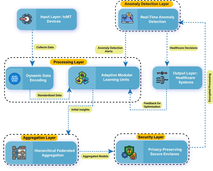
Proposed system architecture illustrating the hierarchical data flow across Input, Processing, Aggregation, Security, and Output layers for healthcare systems.
The upper layers of the framework coordinate secure aggregation and anomaly detection in real time. HFA performs multi-tier aggregation at edge, fog, and cloud levels using data-size weighting and delay-aware coefficients, which mitigates staleness of model updates while maintaining scalability across large deployments. PPSE enforces privacy at the computation layer by executing training and aggregation within hardware-secured enclaves and injecting calibrated differential privacy noise, preventing gradient inversion and inference attacks on sensitive medical data. RTAD operates as a continuous monitoring pipeline, applying sliding windows, dimensionality reduction, covariance-based scoring, and adaptive thresholds to detect anomalies in patient data streams with low latency. This module supports immediate detection of clinically critical events while leveraging continuously updated global models from the federated process.
AFEL modules working
The Adaptive Federated Edge Learning (AFEL) framework is underpinned by modular components that collaborate to ensure efficiency, scalability, and privacy in IoMT-enabled healthcare systems.
Adaptive Modular Learning Units (AMLUs)
AMLUs implement resource-aware local learning on heterogeneous edge nodes. Each AMLU maintains a module-specific resource metric, a resource-constrained training objective, a resource-normalized activation, a resource-proportional fusion rule, and a federated gradient update. The design targets strict device budgets, bounded latency, and stable convergence under heterogeneous feature distributions. The module stack partitions computation across \(m\) hierarchical sub-modules while preserving a common supervision signal.
Let the local dataset be \({\textbf{X}}=\{{\textbf{x}}_1,\dots ,{\textbf{x}}_n\}\), \({\textbf{x}}_i\in {\mathbb {R}}^d\), with target vector \({\textbf{y}}\in {\mathbb {R}}^n\). Computation is partitioned into \(m\) sub-modules \(\{M_1,\dots ,M_m\}\). Equation 1 defines the per-module resource score \(R_j\in {\mathbb {R}}_{>0}\) as
$$\begin{aligned} R_j=\frac{C_j}{T_j}, \end{aligned}$$
(1)
where \(C_j\) denotes available computational capacity for module \(j\) (e.g., effective FLOPs/s) and \(T_j\) denotes expected processing time per inference/training step for module \(j\) (s). The AMLU training objective in Equation 2 is
$$\begin{aligned} \min _{{\textbf{w}}} \;\; \sum _{j=1}^{m} \frac{\Vert {\textbf{X}}_j {\textbf{w}}_j – {\textbf{y}} \Vert _2^{2}}{R_j} + \lambda \Vert {\textbf{w}}_j \Vert _{1}, \end{aligned}$$
(2)
subject to the resource budget in Equation 3,
$$\begin{aligned} \sum _{j=1}^{m} R_j \le R_{\text {max}}, \end{aligned}$$
(3)
where \({\textbf{X}}_j\in {\mathbb {R}}^{n\times d}\) is the module-specific design matrix (e.g., transformed features for \(M_j\)), \({\textbf{w}}_j\in {\mathbb {R}}^{d}\) is the parameter vector of \(M_j\), \({\textbf{w}}=\{{\textbf{w}}_1,\dots ,{\textbf{w}}_m\}\), \(\Vert \cdot \Vert _2\) is the Euclidean norm, \(\Vert \cdot \Vert _1\) is the \(\ell _1\) norm, \(\lambda>0\) is the sparsity regularizer, and \(R_{\text {max}}>0\) is the allowable aggregate resource budget. Equation 2 weights the data-fitting term by \(1/R_j\) to prioritize modules with higher resource scores, while Equation 3 constrains the sum of resource allocations. Equation 4 defines the resource-normalized activation for module \(j\):
$$\begin{aligned} f_j({\textbf{x}}_i)=\sigma \!\left( \frac{{\textbf{x}}_i^{\top }{\textbf{w}}_j}{R_j+\epsilon }\right) , \end{aligned}$$
(4)
where \(\sigma :{\mathbb {R}}\!\rightarrow \!{\mathbb {R}}\) is a differentiable activation (e.g., logistic sigmoid), \({\textbf{x}}_i^{\top }{\textbf{w}}_j\) is the inner product, and \(\epsilon>0\) is a small constant for numerical stability. Equation 5 specifies the fusion of sub-module outputs as a convex combination:
$$\begin{aligned} {\textbf{o}}=\sum _{j=1}^{m}\alpha _j f_j({\textbf{x}}_i), \qquad \alpha _j=\frac{R_j}{\sum _{k=1}^{m} R_k}, \end{aligned}$$
(5)
where \({\textbf{o}}\in {\mathbb {R}}\) is the fused scalar output (extendable to vector outputs per class), \(\alpha _j\in [0,1]\) is the resource-proportional weight, and \(\sum _{j=1}^{m}\alpha _j=1\). Parameter updates follow Equation 6:
$$\begin{aligned} {\textbf{w}}_j^{(t+1)}={\textbf{w}}_j^{(t)}-\eta \,\nabla _{{\textbf{w}}_j}{\mathscr {L}}({\textbf{X}},{\textbf{y}},{\textbf{w}}), \end{aligned}$$
(6)
where \(t\in {\mathbb {N}}\) is the iteration index, \(\eta>0\) is the learning rate, and \({\mathscr {L}}(\cdot )\) is a differentiable local loss (consistent with Equation 2). Gradients are computed on device and subsequently integrated within the federated protocol; the notation \(\nabla _{{\textbf{w}}_j}\) denotes the partial gradient with respect to \({\textbf{w}}_j\).
Hierarchical Federated Aggregation (HFA)
HFA implements a multi-tier aggregation protocol that coordinates device, regional, and global model updates under heterogeneous connectivity and workload conditions. The objective is to reduce communication overhead, control staleness, and preserve convergence properties while operating at scale. The complete multi-tier aggregation protocol with staleness control and delay-aware weighting is specified in Algorithm 1.
Algorithm 1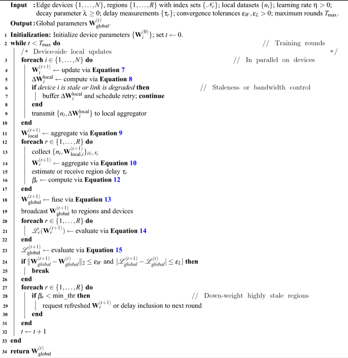
Hierarchical Federated Aggregation (HFA) Protocol
The on-device update rule in Equation 7 performs a first-order step for edge device \(i\in \{1,\dots ,N\}\):
$$\begin{aligned} {\textbf{W}}_i^{(t+1)} = {\textbf{W}}_i^{(t)} – \eta \,\nabla _{{\textbf{W}}_i} {\mathscr {L}}_i\!\left( {\textbf{W}}_i^{(t)}\right) , \end{aligned}$$
(7)
where \({\textbf{W}}_i^{(t)}\in {\mathbb {R}}^{d_w}\) denotes the parameter vector (or vectorized parameter tensor) at iteration \(t\in {\mathbb {N}}\), \(N\) is the number of edge devices, \(\eta>0\) is the learning rate, \({\mathscr {L}}_i:{\mathbb {R}}^{d_w}\!\rightarrow \!{\mathbb {R}}\) is a differentiable local loss for device \(i\), and \(\nabla _{{\textbf{W}}_i}\) is the gradient operator with respect to \({\textbf{W}}_i\). The device-level partial update in Equation 8 records the parameter increment:
$$\begin{aligned} \Delta {\textbf{W}}_i^{\text {local}} = {\textbf{W}}_i^{(t+1)} – {\textbf{W}}_i^{(t)}, \end{aligned}$$
(8)
where \(\Delta {\textbf{W}}_i^{\text {local}}\in {\mathbb {R}}^{d_w}\) is the per-iteration update vector computed locally. Local aggregation across the \(N\) devices uses data-size weights as in Equation 9:
$$\begin{aligned} {\textbf{W}}_{\text {local}}^{(t+1)} = \frac{\sum _{i=1}^{N} n_i \,\Delta {\textbf{W}}_i^{\text {local}}}{\sum _{i=1}^{N} n_i}, \end{aligned}$$
(9)
where \(n_i\in {\mathbb {N}}_{>0}\) denotes the number of training samples (or an equivalent sample-weight proxy) on device \(i\); \({\textbf{W}}_{\text {local}}^{(t+1)}\in {\mathbb {R}}^{d_w}\) is the locally aggregated update. The denominator \(\sum _{i=1}^{N} n_i>0\). Regional aggregation groups devices by region \(r\in \{1,\dots ,R\}\) with index set \({\mathscr {N}}_r\subseteq \{1,\dots ,N\}\). Equation 10 forms the regional aggregate at the fog node:
$$\begin{aligned} {\textbf{W}}_r^{(t+1)} = \frac{\sum _{i \in {\mathscr {N}}_r} n_i \,{\textbf{W}}_{\text {local}, i}^{(t+1)}}{\sum _{i \in {\mathscr {N}}_r} n_i}, \end{aligned}$$
(10)
where \({\textbf{W}}_{\text {local}, i}^{(t+1)}\in {\mathbb {R}}^{d_w}\) denotes the device-\(i\) contribution to the local aggregate (by construction, \({\textbf{W}}_{\text {local}, i}^{(t+1)} \equiv \Delta {\textbf{W}}_i^{\text {local}}\)), \({\textbf{W}}_r^{(t+1)}\in {\mathbb {R}}^{d_w}\) is the regional parameter update, and \(\sum _{i \in {\mathscr {N}}_r} n_i>0\). Global aggregation at the cloud fuses regional updates using regional data-size weights as in Equation 11:
$$\begin{aligned} {\textbf{W}}_{\text {global}}^{(t+1)} = \frac{\sum _{r=1}^{R} n_r \,{\textbf{W}}_r^{(t+1)}}{\sum _{r=1}^{R} n_r}, \end{aligned}$$
(11)
where \(R\in {\mathbb {N}}_{>0}\) is the number of regions, \(n_r=\sum _{i \in {\mathscr {N}}_r} n_i\) is the regional sample count, and \({\textbf{W}}_{\text {global}}^{(t+1)}\in {\mathbb {R}}^{d_w}\) is the global update; \(\sum _{r=1}^{R} n_r>0\). To discount stale contributions, Equation 12 defines a delay-aware coefficient:
$$\begin{aligned} \beta _r = \frac{1}{1 + \lambda \tau _r}, \end{aligned}$$
(12)
where \(\beta _r\in (0,1]\) is dimensionless, \(\tau _r\ge 0\) is the end-to-end communication and processing delay for region \(r\) (s), and \(\lambda \ge 0\) is a tunable scaling parameter controlling the decay rate. The delay-weighted global fusion in Equation 13 integrates \(\beta _r\) into the aggregation:
$$\begin{aligned} {\textbf{W}}_{\text {global}}^{(t+1)} = \frac{\sum _{r=1}^{R} \beta _r n_r \,{\textbf{W}}_r^{(t+1)}}{\sum _{r=1}^{R} \beta _r n_r}, \end{aligned}$$
(13)
where the denominator \(\sum _{r=1}^{R} \beta _r n_r>0\) and each term \(\beta _r n_r\) serves as a joint delay–data weight. Regional and global objectives are defined in Equations 14 and 15. The regional loss aggregates device losses:
$$\begin{aligned} {\mathscr {L}}_r({\textbf{W}}_r) = \sum _{i \in {\mathscr {N}}_r} \frac{n_i}{\sum _{j \in {\mathscr {N}}_r} n_j} \,{\mathscr {L}}_i({\textbf{W}}_i), \end{aligned}$$
(14)
where \({\mathscr {L}}_r:{\mathbb {R}}^{d_w}\!\rightarrow \!{\mathbb {R}}\) is the regional objective. The global loss averages regional objectives:
$$\begin{aligned} {\mathscr {L}}_{\text {global}} = \sum _{r=1}^{R} \frac{n_r}{\sum _{k=1}^{R} n_k} \,{\mathscr {L}}_r({\textbf{W}}_r), \end{aligned}$$
(15)
where \({\mathscr {L}}_{\text {global}}\in {\mathbb {R}}\) is the scalar objective minimized by the protocol.
Dynamic Data Encoding (DDE)
DDE constructs a device-agnostic feature representation that supports distributed optimization under heterogeneous sensing, sampling, and feature spaces. The pipeline comprises standardization, device-specific affine mapping into a universal embedding, cross-device alignment, decorrelation, and quality-weighted fusion, followed by a regularized objective that stabilizes training. The complete device-agnostic encoding workflow with alignment, decorrelation, quality-weighted fusion, and regularized optimization is specified in Algorithm 2.
Algorithm 2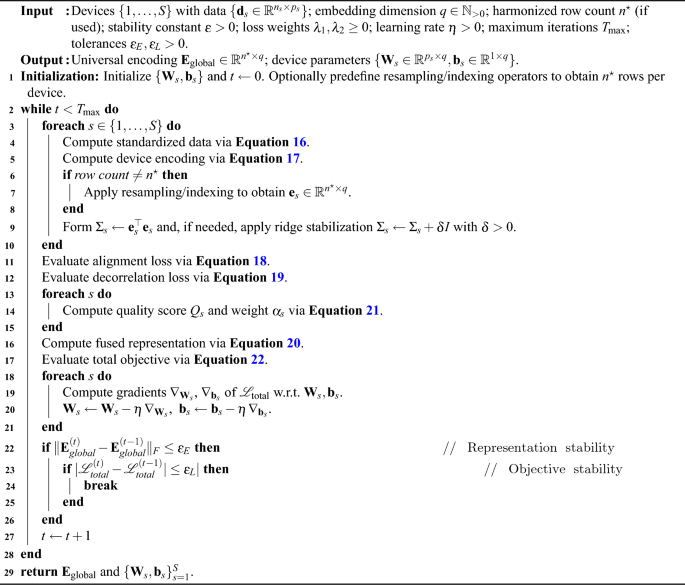
Dynamic Data Encoding (DDE) Workflow
Let \(S\in {\mathbb {N}}_{>0}\) denote the number of Internet of Medical Things devices and \({\textbf{D}}=\{{\textbf{d}}_s\}_{s=1}^{S}\) the set of device-specific data matrices with \({\textbf{d}}_s\in {\mathbb {R}}^{n_s\times p_s}\), where \(n_s\in {\mathbb {N}}_{>0}\) is the sample count and \(p_s\in {\mathbb {N}}_{>0}\) is the feature dimension for device \(s\). Equation 16 defines per-device standardization,
$$\begin{aligned} \tilde{{\textbf{d}}}_s = \frac{{\textbf{d}}_s – \mu _s}{\sigma _s}, \end{aligned}$$
(16)
where \(\tilde{{\textbf{d}}}_s\in {\mathbb {R}}^{n_s\times p_s}\) is the standardized matrix, \(\mu _s\in {\mathbb {R}}^{1\times p_s}\) is the feature-wise mean row vector, and \(\sigma _s\in {\mathbb {R}}^{1\times p_s}\) is the feature-wise standard-deviation row vector (elementwise division). Equation 17 applies a device-specific affine map \(\phi _s:{\mathbb {R}}^{p_s}\rightarrow {\mathbb {R}}^{q}\) to embed the standardized data into a universal \(q\)-dimensional space,
$$\begin{aligned} {\textbf{e}}_s = \phi _s(\tilde{{\textbf{d}}}_s) = \tilde{{\textbf{d}}}_s {\textbf{W}}_s + {\textbf{b}}_s, \end{aligned}$$
(17)
where \({\textbf{e}}_s\in {\mathbb {R}}^{n_s\times q}\) is the encoded matrix for device \(s\), \({\textbf{W}}_s\in {\mathbb {R}}^{p_s\times q}\) is a learnable weight matrix, \({\textbf{b}}_s\in {\mathbb {R}}^{1\times q}\) is a learnable bias row vector broadcast across rows, and \(q\in {\mathbb {N}}_{>0}\) is the universal embedding dimension. Cross-device consistency is encouraged by the pairwise alignment loss in Equation 18,
$$\begin{aligned} {\mathscr {L}}_{\text {align}} = \sum _{s=1}^{S}\sum _{t=1}^{S} \big \Vert {\textbf{e}}_s – {\textbf{e}}_t \big \Vert _{F}^{2}, \end{aligned}$$
(18)
where \(\Vert \cdot \Vert _{F}\) denotes the Frobenius norm and \(\{{\textbf{e}}_s\}_{s=1}^{S}\) are the device encodings. (In practice, row counts are harmonized to a common \(n^{\star }\) by resampling or indexing so that \({\textbf{e}}_s,{\textbf{e}}_t\in {\mathbb {R}}^{n^{\star }\times q}\) for valid subtraction.) To reduce redundancy and enforce whitening, Equation 19 penalizes deviations of second-order statistics from the identity,
$$\begin{aligned} {\mathscr {L}}_{\text {decor}} = \sum _{s=1}^{S} \big \Vert \mathbf {\Sigma }_s – {\textbf{I}} \big \Vert _{F}^{2}, \end{aligned}$$
(19)
where \(\mathbf {\Sigma }_s={\textbf{e}}_s^{\top }{\textbf{e}}_s\in {\mathbb {R}}^{q\times q}\) is the unnormalized second-moment matrix of \({\textbf{e}}_s\) and \({\textbf{I}}\in {\mathbb {R}}^{q\times q}\) is the identity matrix. The device encodings are combined by the quality-weighted fusion in Equation 20,
$$\begin{aligned} {\textbf{E}}_{\text {global}} = \sum _{s=1}^{S} \alpha _s {\textbf{e}}_s, \end{aligned}$$
(20)
where \({\textbf{E}}_{\text {global}}\in {\mathbb {R}}^{n^{\star }\times q}\) is the fused encoding (after row harmonization) and \(\alpha _s\in [0,1]\) are device weights that sum to one. Equation 21 specifies \(\alpha _s\) via quality scores \(Q_s\),
$$\begin{aligned} \alpha _s = \frac{Q_s}{\sum _{t=1}^{S} Q_t}, \quad Q_s = \frac{1}{\big \Vert \mathbf {\Sigma }_s – {\textbf{I}} \big \Vert _{F} + \epsilon }, \end{aligned}$$
(21)
where \(Q_s\in {\mathbb {R}}_{>0}\) is the inverse-whitening-deviation score for device \(s\), \(\epsilon>0\) ensures numerical stability, and \(\sum _{t=1}^{S}Q_t>0\) guarantees a valid normalization. The total objective in Equation 22 couples alignment, decorrelation, and Tikhonov regularization of the fused representation,
$$\begin{aligned} {\mathscr {L}}_{\text {total}} = {\mathscr {L}}_{\text {align}} + \lambda _{1}\,{\mathscr {L}}_{\text {decor}} + \lambda _{2}\,\big \Vert {\textbf{E}}_{\text {global}} \big \Vert _{F}^{2}, \end{aligned}$$
(22)
where \(\lambda _{1}\ge 0\) and \(\lambda _{2}\ge 0\) are hyperparameters that control the trade-off between cross-device alignment, feature decorrelation, and magnitude regularization of \({\textbf{E}}_{\text {global}}\). The Frobenius term \(\Vert {\textbf{E}}_{\text {global}}\Vert _{F}^{2}\) equals the sum of squared entries of the fused encoding and stabilizes optimization.
Privacy-Preserving Secure Enclaves (PPSE)
PPSE formalizes computation over protected representations inside hardware-backed trusted execution environments. The mechanism uses an affine masking transform for inputs, enclave-confined linear algebra for inference and training, encrypted aggregation of updates, and calibrated differential privacy noise for release.
Algorithm 3
Privacy-Preserving Secure Enclaves (PPSE) Training and Aggregation
Let \({\textbf{X}}=\{{\textbf{x}}_i\}_{i=1}^{n}\) with \({\textbf{x}}_i\in {\mathbb {R}}^{d}\) denote the input samples (\(n\) samples, \(d\) features). Equation 23 defines the enclave-side affine masking transform
$$\begin{aligned} {\mathscr {E}}({\textbf{x}}_i)={\textbf{x}}_i^{\top }{\textbf{K}}+{\textbf{r}}_i^{\top }, \end{aligned}$$
(23)
where \({\textbf{K}}\in {\mathbb {R}}^{d\times d}\) is a full-rank secret key matrix known only inside the enclave, and \({\textbf{r}}_i\in {\mathbb {R}}^{d}\) is a per-sample random mask (zero-mean, enclave-generated). Stackwise, \({\mathscr {E}}({\textbf{X}})={\textbf{X}}{\textbf{K}}+{\textbf{R}}\in {\mathbb {R}}^{n\times d}\) with \({\textbf{R}}=[{\textbf{r}}_1,\dots ,{\textbf{r}}_n]^{\top }\). Given model parameters \({\textbf{W}}\in {\mathbb {R}}^{d\times o}\) (\(o\) outputs), Equation 24 defines masked-domain inference:
$$\begin{aligned} {\mathscr {E}}({\textbf{y}})={\mathscr {E}}({\textbf{X}})\,{\textbf{W}}, \end{aligned}$$
(24)
where \({\mathscr {E}}({\textbf{y}})\in {\mathbb {R}}^{n\times o}\) are masked outputs. Expanding Equation 24 yields Equation 25:
$$\begin{aligned} {\mathscr {E}}({\textbf{y}})=({\textbf{X}}{\textbf{K}}+{\textbf{R}})\,{\textbf{W}}, \end{aligned}$$
(25)
where \({\textbf{X}}{\textbf{K}}\in {\mathbb {R}}^{n\times d}\) and \({\textbf{R}}{\textbf{W}}\in {\mathbb {R}}^{n\times o}\). Equation 26 recovers plaintext predictions using the enclave-held inverse \({\textbf{K}}^{-1}\):
$$\begin{aligned} {\mathscr {D}}({\mathscr {E}}({\textbf{y}}))=\big ({\mathscr {E}}({\textbf{y}})-{\textbf{R}}{\textbf{W}}\big )\,{\textbf{K}}^{-1}, \end{aligned}$$
(26)
where \({\mathscr {D}}(\cdot )\) denotes the de-masking map and \({\textbf{K}}^{-1}\in {\mathbb {R}}^{d\times d}\) exists by full rank. Let \(N\in {\mathbb {N}}_{>0}\) be the number of collaborating nodes and \({\mathscr {E}}({\textbf{y}}_i^{(t)})\in {\mathbb {R}}^{d_w}\) be the masked update vector from node \(i\) at iteration \(t\) (\(d_w\) parameters). Equation 27 defines additive aggregation in the masked domain:
$$\begin{aligned} {\mathscr {E}}({\textbf{y}}_{\text {agg}}^{(t)})=\sum _{i=1}^{N}{\mathscr {E}}({\textbf{y}}_i^{(t)}), \end{aligned}$$
(27)
where the sum is elementwise over parameter coordinates. Equation 28 applies enclave de-masking:
$$\begin{aligned} {\textbf{y}}_{\text {agg}}^{(t)}={\mathscr {D}}\!\left( {\mathscr {E}}({\textbf{y}}_{\text {agg}}^{(t)})\right) , \end{aligned}$$
(28)
yielding the plaintext aggregate update \({\textbf{y}}_{\text {agg}}^{(t)}\in {\mathbb {R}}^{d_w}\) only within the enclave boundary. Let \({\mathscr {L}}:{\mathbb {R}}^{n\times o}\times {\mathbb {R}}^{n\times o}\rightarrow {\mathbb {R}}\) be a differentiable loss, \({\textbf{Y}}\in {\mathbb {R}}^{n\times o}\) be labels (e.g., one-hot or continuous), and \(\eta>0\) be the learning rate. Using masked operands, Equation 29 states the gradient in the masked domain:
$$\begin{aligned} \nabla {\mathscr {L}}\big ({\mathscr {E}}({\textbf{X}}),{\mathscr {E}}({\textbf{W}})\big ) ={\mathscr {E}}\!\left( {\textbf{X}}^{\top }\big ({\mathscr {E}}({\textbf{X}})\,{\textbf{W}}-{\mathscr {E}}({\textbf{Y}})\big )\right) , \end{aligned}$$
(29)
where \({\mathscr {E}}({\textbf{W}})\) and \({\mathscr {E}}({\textbf{Y}})\) denote masked parameters and masked labels, respectively; \({\textbf{X}}^{\top }\big (\cdot \big )\in {\mathbb {R}}^{d\times o}\) matches \({\textbf{W}}\)’s shape. Equation 30 applies the masked-domain update:
$$\begin{aligned} {\mathscr {E}}\!\left( {\textbf{W}}^{(t+1)}\right) ={\mathscr {E}}\!\left( {\textbf{W}}^{(t)}\right) -\eta \,\nabla {\mathscr {L}}\big ({\mathscr {E}}({\textbf{X}}),{\mathscr {E}}({\textbf{W}})\big ), \end{aligned}$$
(30)
where \({\textbf{W}}^{(t)}\in {\mathbb {R}}^{d\times o}\) is the parameter matrix at iteration \(t\). To enforce record-level privacy during aggregation, Equation 31 injects calibrated Gaussian noise in the masked domain:
$$\begin{aligned} {\mathscr {E}}({\textbf{y}}_{\text {agg}}^{(t)}) \leftarrow {\mathscr {E}}({\textbf{y}}_{\text {agg}}^{(t)}) + \Delta {\textbf{N}}, \qquad \Delta {\textbf{N}}\sim {\mathscr {N}}\!\left( {\textbf{0}},\,\sigma ^{2}{\textbf{I}}\right) , \end{aligned}$$
(31)
where \(\Delta {\textbf{N}}\in {\mathbb {R}}^{d_w}\), \(\sigma ^{2}>0\) is the noise variance, and \({\textbf{I}}\) is the \(d_w\times d_w\) identity matrix. The enclave-anchored training objective in Equation 32 minimizes the expected plaintext loss under masking:
$$\begin{aligned} \min _{{\textbf{W}}\in {\mathbb {R}}^{d\times o}} \;\; {\mathbb {E}}_{{\mathscr {E}}}\!\left[ \,{\mathscr {L}}\!\big ({\mathscr {D}}({\mathscr {E}}({\textbf{X}})\,{\textbf{W}}),\,{\textbf{Y}}\big )\right] , \end{aligned}$$
(32)
subject to the masking constraint in Equation 33:
$$\begin{aligned} \big \Vert {\mathscr {E}}({\textbf{x}}_i)-{\textbf{x}}_i^{\top }\big \Vert _{2}\le \epsilon , \quad \forall i\in \{1,\dots ,n\}, \end{aligned}$$
(33)
where \(\epsilon>0\) bounds per-sample deviation between masked and plaintext representations (measured in \({\mathbb {R}}^{1\times d}\)). Constraint \(\epsilon\) sets a limit on masking distortion to preserve numerical stability of downstream linear algebra while maintaining confidentiality within the enclave. The symbols, variables, and parameters used across the Adaptive Federated Edge Learning framework are summarized in Table 3.
Table 3 Notation summary of symbols and parameters used in the Adaptive Federated Edge Learning (AFEL) framework.Real-Time Anomaly Detection (RTAD)
RTAD provides continuous assessment of streaming clinical signals under strict latency constraints. The pipeline comprises (i) temporal windowing, (ii) feature projection, (iii) covariance-based scoring, (iv) adaptive thresholding, (v) density-aware clustering, (vi) priority assignment, and (vii) stability optimization.
Let the data stream at time \(t\in {\mathbb {R}}_{\ge 0}\) be \({\textbf{S}}(t)=\{{\textbf{s}}_{i}(t)\}_{i=1}^{n}\) with \({\textbf{s}}_{i}(t)\in {\mathbb {R}}^{d}\) (\(n\) samples, \(d\) features). Equation 34 defines the temporal window
$$\begin{aligned} {\mathscr {W}}_{t}=\{{\textbf{s}}_{i}(\tau )\mid \tau \in [t-\Delta t,\,t]\}, \end{aligned}$$
(34)
where \(\Delta t>0\) is the window length (s). The windowed matrix in Equation 35 stacks observations:
$$\begin{aligned} {\textbf{M}}_{t}=\begin{bmatrix} {\textbf{s}}_{1}(t-\Delta t) & \cdots & {\textbf{s}}_{n}(t-\Delta t)\\ \vdots & \ddots & \vdots \\ {\textbf{s}}_{1}(t) & \cdots & {\textbf{s}}_{n}(t) \end{bmatrix}\!, \end{aligned}$$
(35)
with \({\textbf{M}}_{t}\in {\mathbb {R}}^{w\times n d}\) or, equivalently, reshaped to \({\mathbb {R}}^{n\times d}\) after temporal aggregation; \(w\) is the number of sampled instants in \([t-\Delta t,t]\). Dimensionality reduction uses a linear map \(\Phi :{\mathbb {R}}^{n\times d}\rightarrow {\mathbb {R}}^{n\times k}\) with \(k\in {\mathbb {N}}_{>0}\). Equation 36 defines the (unnormalized) covariance proxy,
$$\begin{aligned} \mathbf {\Sigma }_{t}={\textbf{M}}_{t}^{\top }{\textbf{M}}_{t}, \end{aligned}$$
(36)
where \(\mathbf {\Sigma }_{t}\in {\mathbb {R}}^{d\times d}\). The projection in Equation 37 applies \({\textbf{U}}_{t}\),
$$\begin{aligned} {\textbf{F}}_{t}=\Phi ({\textbf{M}}_{t})={\textbf{U}}_{t}{\textbf{M}}_{t}, \end{aligned}$$
(37)
where \({\textbf{U}}_{t}\in {\mathbb {R}}^{k\times d}\) contains the top-\(k\) eigenvectors of a covariance estimate compatible with \(\mathbf {\Sigma }_{t}\), and \({\textbf{F}}_{t}=[{\textbf{f}}_{1}(t),\dots ,{\textbf{f}}_{n}(t)]^{\top }\in {\mathbb {R}}^{n\times k}\) are projected features. Anomaly scoring uses a quadratic form under the inverse covariance metric. Equation 38 defines
$$\begin{aligned} A_{i}(t)=\sqrt{({\textbf{f}}_{i}(t)-\varvec{\mu }_{t})^{\top }{\textbf{C}}_{t}^{-1}({\textbf{f}}_{i}(t)-\varvec{\mu }_{t})}, \end{aligned}$$
(38)
where \({\textbf{f}}_{i}(t)\in {\mathbb {R}}^{k}\) is the \(i\)-th projected vector, \(\varvec{\mu }_{t}\in {\mathbb {R}}^{k}\) is the sample mean of rows of \({\textbf{F}}_{t}\), and \({\textbf{C}}_{t}\in {\mathbb {R}}^{k\times k}\) is a positive-definite covariance estimate (e.g., shrinkage of \(\operatorname {cov}({\textbf{F}}_{t})\)). Adaptive thresholding in Equation 39 sets
$$\begin{aligned} \tau (t)=\mu _{A}(t)+\alpha \,\sigma _{A}(t), \end{aligned}$$
(39)
where \(\mu _{A}(t)\in {\mathbb {R}}\) and \(\sigma _{A}(t)\in {\mathbb {R}}_{>0}\) are the mean and standard deviation of \(\{A_{i}(t)\}_{i=1}^{n}\), and \(\alpha>0\) controls sensitivity. Context modeling uses clustering. Equation 40 defines cluster \(C_{j}(t)\),
$$\begin{aligned} C_{j}(t)=\{{\textbf{f}}_{i}(t)\mid \Vert {\textbf{f}}_{i}(t)-{\textbf{c}}_{j}(t)\Vert _{2}<\epsilon _{j}\}, \end{aligned}$$
(40)
where \({\textbf{c}}_{j}(t)\in {\mathbb {R}}^{k}\) is the centroid and \(\epsilon _{j}>0\) is the inclusion radius. Equation 41 updates \(\epsilon _{j}\) from intra-cluster dispersion,
$$\begin{aligned} \epsilon _{j}=\frac{\sum _{{\textbf{f}}_{i}\in C_{j}(t)} \Vert {\textbf{f}}_{i}(t)-{\textbf{c}}_{j}(t)\Vert _{2}}{|C_{j}(t)|}, \end{aligned}$$
(41)
where \(|C_{j}(t)|\in {\mathbb {N}}_{\ge 0}\) is the cluster cardinality. Cluster density in Equation 42 is
$$\begin{aligned} D_{j}(t)=\frac{|C_{j}(t)|}{\operatorname {Volume}(C_{j}(t))}, \end{aligned}$$
(42)
where \(\operatorname {Volume}(C_{j}(t))>0\) denotes a \(k\)-dimensional volume proxy (e.g., hypersphere with radius \(\epsilon _{j}\)). Priority assignment uses ordinal levels. Equation 43 maps decisions to \(\{1,2,3\}\),
$$\begin{aligned} {\mathscr {R}}(t)={\left\{ \begin{array}{ll} 3, & A_{i}(t)>\beta \,\tau (t),\\ 2, & \tau (t)
(43)
where \(\beta>1\) scales the high-priority threshold and \({\mathscr {R}}(t)\in \{1,2,3\}\) is the assigned priority for the current assessment. Temporal stability is quantified by entropy in Equation 44,
$$\begin{aligned} H(t)=-\sum _{k=1}^{K} p_{k}(t)\,\log p_{k}(t), \end{aligned}$$
(44)
where \(K\in {\mathbb {N}}_{>0}\) is the number of active clusters and \(p_{k}(t)\in [0,1]\) is the proportion of detected anomalies in \(C_{k}(t)\) with \(\sum _{k}p_{k}(t)=1\). The stability objective in Equation 45 balances entropy and score variation,
$$\begin{aligned} \max \;\; \sum _{t=1}^{T} H(t)-\gamma \sum _{t=1}^{T}\big |A(t)-A(t-1)\big |, \end{aligned}$$
(45)
where \(T\in {\mathbb {N}}_{>0}\) is the horizon, \(\gamma>0\) is a smoothness coefficient, and \(A(t)=\frac{1}{n}\sum _{i=1}^{n}A_{i}(t)\). The RTAD loss in Equation 46 integrates pointwise and contextual penalties,
$$\begin{aligned} \min _{\Phi ,\,\tau ,\,C} \;\; {\mathscr {L}}_{\text {RTAD}}&=\sum _{t=1}^{T}\Bigg [\sum _{i=1}^{n}\big (A_{i}(t)-\tau (t)\big )^{2} +\lambda \sum _{j=1}^{K}\big (D_{j}(t)-\delta \big )^{2}\Bigg ], \end{aligned}$$
(46)
where \(\lambda \ge 0\) controls the contextual penalty, \(\delta>0\) is the density threshold, and the optimization variables are the projection \(\Phi\), threshold function \(\tau (\cdot )\), and cluster assignment \(C=\{C_{j}(t)\}\).