
Study design and population sample
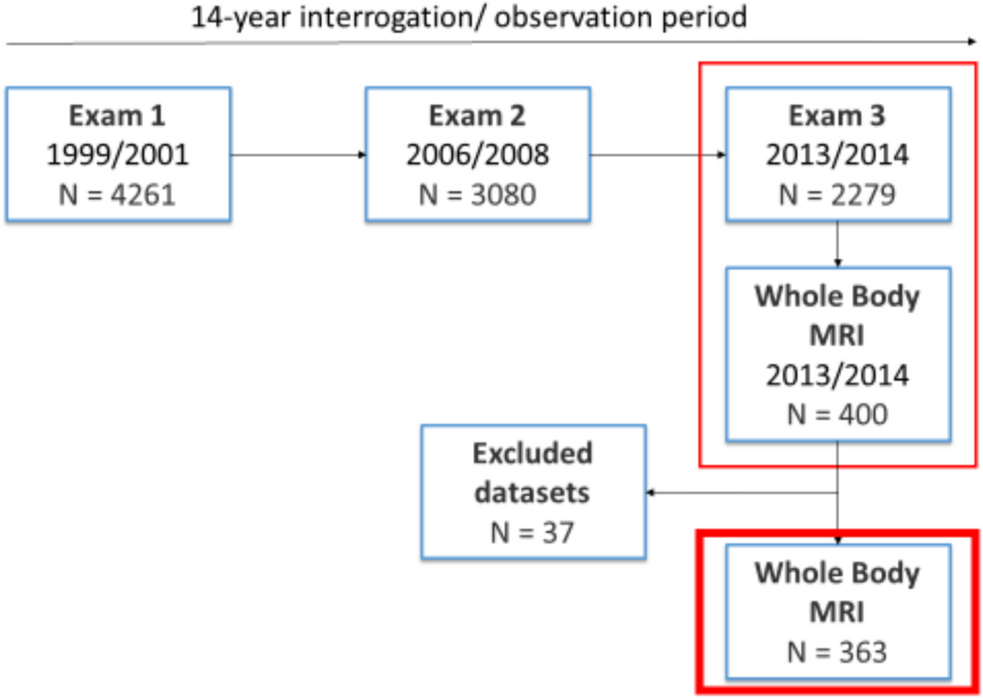
Participants were derived from the “Cooperative Health Research in the Region of Augsburg” (KORA) S4-study (N = 4261) with a baseline examination in 1999 to 2001 (exam 1), a follow-up examination in 2006 to 2008 (exam 2) and a second follow-up in 2013 and 2014 (exam 3). Hereof, 400 participants received a whole-body MRI during exam 3 [21].
Participants were considered eligible for inclusion if they were willing to undergo a whole-body MRI and were classified into one of the following groups based on health assessment: prediabetes, diabetes, or control. Individuals were excluded from the study if they were older than 72 years, had a history (self-reported or confirmed) of stroke, myocardial infarction, or revascularization, or had contraindications for MRI such as a cardiac pacemaker, implantable defibrillator, cerebral aneurysm clip, neural stimulator, ear implants, ocular foreign bodies, or any other implanted device. Additional exclusion criteria included pregnancy or breastfeeding, claustrophobia, known allergies to gadolinium-based contrast agents, or a serum creatinine level of ≥ 1.3 mg/dL [22].
Approval was given by the institutional review board of the Ludwig Maximilian’s University Munich (Germany). Written consent was obtained from every participating subject.
MR imaging protocol
During exam 3 in total 400 whole-body MR examinations were performed on a 3 Tesla scanner (Magnetom Skyra, Siemens Healthcare, Erlangen, Germany). A detailed description of the technical procedure as well as imaging protocols can be found elsewhere [22].
Briefly summarized, the musculoskeletal protocol embedded a dual-echo Dixon sequence (matrix: matrix: 256 × 256, field of view (FOV): 488 × 716 mm, echo time (TE) 1.26 ms and 2.49 ms, repetition time (TR): 4.06 ms, partition segments: 1.7 mm, flip angle: 9°) and a T2w single shot fast spin echo (SS-FSE) sequence (matrix: matrix: 320 × 200, field of view (FOV): 296 × 380 mm, echo time (TE) 91 ms, repetition time (TR): 1000 ms, partition segments: 5 mm, flip angle: 131°) [23].
A 2-point T1-weighted VIBE sequences (repetition time (TR): 4.06 ms; time to echo (TEs): 1.26 ms and 2.49 ms; flip angle 4°; slice thickness 1.7 mm) was used to determine bone marrow fat fraction (BMFF) in lumbar vertebrae L1 and L2 [24]. T2*-corrected, multi-echo 3D-gradient-echo Dixon-based sequence (repetition time (TR): 8.90 ms; TEs: 1.23 ms, 2.46 ms, 3.69 ms 4.92 ms, 6.15 ms and 7.38 ms; flip angle 4°, slice thickness 4 mm) was performed to measure skeletal muscle fat fraction (SMFF) in lumbar vertebrae L3 [25]. Based on a VIBE-Dixon sequence (TR: 4.06 ms; TEs: 1.26, 2.49 ms; flip angle 9°; slice thickness: 1.7 mm) VAT and SAT were quantified on a calculated fat-selective tomogram. VAT and SAT together form total adipose tissue (TAT) [22].
Body composition analysis was performed by determining MR imaging biomarkers of bone marrow fat fraction (BMFF), skeletal muscle fat fraction (SMFF) and visceral (VAT) and subcutaneous adipose tissue (SAT). Osteopenia and osteoporosis, characterized by reduced bone mineral density (BMD), have been described as “bone obesity,” with recent data suggesting that increased bone marrow fat fraction (BMFF) inversely correlates with BMD, thus making BMFF a potential imaging biomarker for the osteopenic phenotype [7]. Phenotypic assignment to the OSO complex was performed based on these components.
Outcome definition of osteosarcopenic obesity subgroups
The sex-specific median was calculated for the biomarkers of bone marrow fat fraction (BMFF), skeletal muscle fat fraction (SMFF) and total adipose tissue (TAT). A value greater than the median BMFF, SMFF or TAT has been classified as an osteopenic, sarcopenic or obese phenotype, whereas a value less-than-equal was classified as a healthy phenotype (Table 1).
Table 1 Phenotypic subgroups of osteosarcopenic obesityRisk factor measurements of physical inactivity
In our cohort, physical inactivity was measured via a standardized questionnaire at exam 1 (1999–2001), exam 2 (2006–2008) and exam 3 (2013–2014) using a single-choice question with a four graded answer as previously described [23].
Exercise inactivity per week
a)
No physical activity
b)
irregularly for ≤ 1 h
c)
regularly for ≥ 1 h
d)
regularly for ≥ 2 h
Referring to a previous study [23], this was used to calculate a dichotomous variable with.
a)
physical activity irregularly ≤ 1 h per week
b)
physical activity regularly ≥ 1 h per week.
Furthermore, two different longitudinal variables were generated: The first longitudinal variable was calculated of physical activity performed regularly ≥ 1 h over the time course of 14 years with.
a)
three-times (exam 1, exam 2 and exam 3)
b)
two-times (at two exams out of three)
c)
one-time (at one exam out of three)
d)
never (in any of the three exams).
The second longitudinal variable was gathered by summing up physical inactivity categories of all three exams with one point for physical activity regularly for ≥ 2 h, two points for physical activity regularly ≥ 1 h, 3 points for physical activity irregularly for ≤ 1 h and 4 points for no physical activity. This results in in values from 3 to 12; with a value of 3 indicating physical activity regularly performed for ≥ 2 h per week during all three examinations and a value of 12 representing no physical activity at any of the three exams [23].
Furthermore, information on work inactivity, as well as levels of inactivity related to walking and cycling, were collected through a four-level question for each category.
Work inactivity
a)
no relevant physical labor
b)
light physical labor
c)
moderate physical labor
d)
heavy physical labor
Walk inactivity (in minutes (min) per day)
a)
15 min
b)
15 to 30 min
c)
30 to 60 min
d)
>60 min
Cycling inactivity (in minutes per day)
a)
15 min
b)
15 to 30 min
c)
30 to 60 min
d)
>60 min
Lower back pain
Lower back pain was investigated via a single-choice question with a five graded answer:
a)
no back pain
b)
little back pain
c)
moderate back pain
d)
strong back pain
e)
very strong back pain
We chose a descriptive method to assess lower back pain using a single-choice question with five graded response options (ranging from “no” to “very strong” back pain) in order to capture not only pain intensity but also subjective differences in pain perception. This graded self-assessment allows for a practical and real-life relevant classification of the symptoms, particularly in chronic conditions such as osteosarcopenic obesity.
Covariates
The division into healthy, prediabetic, and diabetic was determined on the basis of the oral glucose tolerance test (OGTT) and fasting glucose levels: Impaired Fasting Glucose (IFG): FPG 5.6–6.9 mmol/L and Impaired Glucose Tolerance (IGT): OGTT 7.8–11.0 mmol/L. Subjects were categorized as having prediabetes if they met the criteria for IFG and/or IGT. However, if either the IFG or IGT criteria for diabetes mellitus were fulfilled (i.e., Diabetes Mellitus: FPG ≥ 7.0 mmol/L and/or OGTT ≥ 11.1 mmol/L and Healthy Controls: FPG < 5.6 mmol/L and OGTT < 7.8 mmol/L), the subject was classified as having diabetes mellitus. This approach ensured a clear and consistent classification based on standard diagnostic thresholds.
BMI was calculated as the subjects’ weight in kilograms (kg)/height in meters squared (m2). A blood pressure ≥ 140/90 mmHg was defined as hypertension. Smoking status was recorded as a single choice question with three options: current smoker, former smoker, or never smoker. A detailed overview has been published elsewhere [26].
Statistical analysis
Descriptive characteristics of participants during last examination are provided as means with standard deviations for continuous measurements and as absolute numbers and proportions for categorical measurements. Venn and bar diagrams were used to illustrated distribution of OSO subgroups. The correlations of OSO subgroups with proportion of irregular physical activity and back pain were evaluated by chi-square test, respectively.
Associations between physical inactivity and OSO were assessed by multinomial logistic regression models adjusted for age, sex, smoking, hypertension, and diabetes mellitus. Relative risk ratios (RRR) together with 95% confidence intervals (95% CI) were calculated. Physical active and healthy subjects were considered as reference group.
A p-value of < 0.05 was considered statistically significant. Statistical analyses were performed using Stata 16.1 (Stata Corporation, College Station, TX, U.S.A.).