
This study has been pre-registered (NCT04969549, https://clinicaltrials.gov/study/NCT04969549 and https://osf.io/rhxm2). A more detailed description of the methods can be found in the Supplementary Material.
Sample
The Brazil-England Study on Mechanisms and Response Predictors of iTBS Treatment (BRAEN-MAP study) was conducted in the Instituto de Psiquiatria do Hospital das Clínicas da Faculdade de Medicina da Universidade de São Paulo between August 2021 and November 2022. Participants were recruited through social media advertisement, Google Ads and flyers posted on bulletin boards at the Hospital das Clínicas. 52 individuals took part in the study (see Supplements for sample size justification). 3 participants discontinued the study after two weeks of iTBS treatment, resulting in a final sample size of 49 participants (Gender: 41 female, 8 male; ethnicity: 7 black, 12 pardo (mixed ethnic ancestry), 27 white, and 2 yellow/Asian (one not declared)). Participants were eligible for the study if they were between 18 and 65 years of age, had a Hamilton Depression Rating Scale (HAM-D) [27] score of 14 or above, and met the criteria for a current diagnosis of major depressive disorder as confirmed by the Mini-International Neuropsychiatric Interview (MINI) [28] (not necessarily treatment-resistant depression). Exclusion criteria were current diagnosis of substance dependence, severe clinical or neurological disorders, suicidal ideation, psychotic symptoms, or manic symptoms (Young Mania Rating Scale > 8). Patients with contraindications to TMS or MRI, such as metallic implants or a diagnosis of epilepsy, were excluded from the study. Treatment-resistant depression (usually defined as at least two unsuccessful prior treatment attempts) was not an inclusion or exclusion criterion in this study. 30 of the participants were taking psychoactive medication (see Supplementary Table 1). Demographic and clinical baseline characteristics are included in Table 1. Participants had experienced an average of 6 depressive episodes (SD = 11.0), with the current episode lasting around 36.5 months (SD = 58.3)(see Figure S12). The study was approved by the National Ethics Committee in Brazil (CAEE: 52384921.6.0000.0068), and all participants gave written informed consent according to the Declaration of Helsinki.
Table 1 Baseline characteristics.Procedure
Participants were invited to a ‘Baseline’ experimental session which included clinical assessments, a behavioural task (Facial Expression Recognition Task (FERT)), and an MRI scan, including a structural T1 scan and task fMRI (Fig. 1). After completion of the Baseline session, participants started iTBS treatment. TMS treatment consisted of 20 sessions of iTBS delivered over the course of four weeks (Monday to Friday). The protocol included 1,800 pulses per session applied at 100% resting motor threshold. The resting motor threshold was defined as the lowest intensity required to elicit a contraction in the first dorsal interosseous muscle in 3 out of 5 TMS pulses over the motor hotspot. The resting motor threshold was assessed on the first two days of each treatment week. If there was a significant change of more than 5 percentage points between the two days, the motor threshold was reassessed on the third day (or even further), until there was no significant variation from one day to the next.
Fig. 1: Experimental procedure.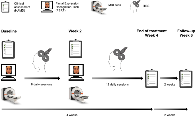
Participants completed a Baseline experimental session involving clinical assessments, the Facial Expression Recognition Task, and an MRI scan (including task fMRI). After ~8 daily iTBS sessions, the second experimental session (Week 2) was conducted which was identical to the Baseline session. Participants received a total of 20 iTBS sessions over 4 weeks. Clinical assessments were obtained weekly throughout the treatment period, including at the end of treatment (Week 4), and at follow-up (Week 6). The primary outcome measure timepoint was end of treatment (Week 4). Figure adapted from [67].
After around 8 iTBS sessions, participants completed a second experimental session (‘Week 2’) identical to the Baseline session. Due to practical considerations, the exact number of iTBS sessions varied between 7 and 10 which was controlled for in the analysis (4/37/4/4 participants received 7/8/9/10 iTBS sessions before the second experimental session). Participants completed the clinical assessments again at the end of treatment (Week 4), and at a two-week follow-up (Week 6).
Clinical outcome measures
The primary outcome measure was the change in Hamilton Depression Rating Scale (17-item version)(HAM-D) [27] score from Baseline to the end of treatment (Week 4). Clinical Response was defined as a categorical variable reflecting a reduction in HAM-D score from Baseline to Week 4 by at least 50% (‘Responders’), or less than 50% (‘Non-Responders’). To increase statistical power [29], HAM-D change was also coded as a continuous variable, HAM-D Improvement (i.e. Baseline HAM-D – Week 4 HAM-D, a positive value indicates symptom reduction). The difference in HAM-D scores (rather than percentage change in HAM-D scores) was used due to statistical advantages [30] (Baseline HAM-D scores were controlled for, see analysis section).
The HAM-D score at Week 4 was missing for one participant (Week 6 score was available). Reduction in HAM-D score at Week 4 was estimated by fitting an exponential decay function to the remaining HAM-D reduction scores for this participant (Week 0–3).
Facial expression recognition task (FERT)
The FERT was adapted from Young et al. [18]. The task protocol included 250 trials in total, separated into two blocks of 62 and two blocks of 63 trials. On each trial, a face with an emotional expression was presented for 500 ms. Participants were instructed to indicate the emotion of the face as quickly and accurately as possible by clicking onto the corresponding key on a labelled keyboard. Emotions included happy, surprise, anger, fear, sadness, disgust and neutral. Each emotion (apart from neutral) was presented at 10 different intensities, by four different actors (i.e. 4 ×10 images per emotion). Ten neutral faces were included as well.
As outcome measures, four Positive Bias measures were defined based on different performance metrics. These performance metrics were calculated separately for positive (happiness, surprise) and negative emotions (fear, anger, sadness, disgust). Positive Bias measures were defined as the ratio of each performance metric for positive vs. negative stimuli, and were log-transformed to ensure symmetry and interpretability. All Positive Bias measures were defined in a way so that a higher value indicates a more positive bias.
Positive bias unbiased hit rate
The Unbiased Hit Rate (based on signal-detection theory [31]) is a measure for how accurately participants identified each emotion. It takes into account how often each emotion was correctly identified, but also how often each emotion was chosen incorrectly:
$$ {Unbiased}\,{Hit}\,{Rate}=\\ {percentage}\,{emotion}\,{correctly}\,{identified}* \,\frac{{number}\,{of}\,{trials}\,{emotion}\,{correctly}\,{chosen}}{{number}\,{of}\,{trials}\,{emotion}\,{chosen}}$$
The measure of interest was Positive Bias Unbiased Hit Rate, defined as the log-transformed ratio of Unbiased Hit Rate averaged across positive emotions (happy, surprise) divided by averaged Unbiased Hit Rate for negative emotions (fear, sadness, anger, disgust).
Positive bias reaction time
For each emotion, the median reaction time was calculated by taking the median across all trials in which the emotion was correctly identified. Positive Bias Reaction Time was calculated as the log-transformed ratio of the median reaction time for negative emotions divided by the median reaction time for positive emotions.
Positive bias efficiency
Efficiency combines accuracy and speed into one measure, by dividing Unbiased Hit Rate by the median reaction time. Positive Bias Efficiency was defined as the log-transformed ratio of Efficiency for positive emotions divided by Efficiency for negative emotions.
Positive bias misclassification
The number of Misclassifications for each emotion was the number of times the emotion has been chosen incorrectly. Positive Bias Misclassification was defined as the log-transformed ratio of Misclassifications as positive emotions, divided by the number of Misclassifications as negative emotions (this is independent of whether the correct emotion was positive or negative). In contrast to the above measures which capture a bias in the ability to recognise emotions, this measure captures a bias in the response criterion (i.e. a general tendency to indicate a positive or negative emotion), and has been found to be sensitive to the effects of antidepressant medication [21].
FERT data were analysed in R (version 4.1.1) [32]. To test whether changes in positive bias were related to Clinical Response, an ANOVA was conducted for each positive bias measure as dependent variable, Time (Baseline vs. Week 2) as within-subject factor and Clinical Response (Responders vs. Non-Responders) as between-subject factor. Significant findings were cross-validated using a logistic regression analysis predicting Clinical Response. Change in positive bias was included as regressor of interest, and Baseline HAM-D, Age, Gender, use of Psychoactive Medication (yes/no) and Number of iTBS Sessions (before ‘Week 2’ time point) as control regressors. Significant interaction effects of Clinical Response and Time were followed up using an ANOVA to test whether the effect was driven by a specific emotion (change in positive bias as dependent variable, Emotion (Happiness, Surprise, Fear, Anger, Sadness, Disgust) and Time as within-subject factors, and Clinical Response as between-subject factor).
To test whether changes in positive bias might predict HAM-D Improvement as continuous variable, linear regression analyses were performed separately for each positive bias measure, using HAM-D Improvement as dependent variable, and change in positive bias as predictor. Baseline HAM-D, Age, Gender, Psychoactive Medication and Number of iTBS Sessions were included as control regressors.
Reported p-values are either uncorrected (‘p’), or corrected for multiple comparisons (four comparisons since there were four positive bias metrics) using Bonferroni correction (‘pcorr’).
Emotional faces fMRI task
Participants completed a gender discrimination task which involved passive processing of emotional facial expressions [19]. The task included four blocks of happy faces and four blocks of fearful faces, which were interleaved by nine blocks displaying only a fixation cross. In total, 120 fearful and 120 happy faces were presented for 100 ms each. Participants were instructed to report the gender of the presented face via button press. Although the emotional expression of the faces is irrelevant to the task, the task has been shown to activate emotional processing networks [9, 19].
For each participant, the median reaction time (RT) was calculated separately for happy faces and fearful faces (correct responses only). Accuracy was defined as the percentage of correct responses for happy or fearful faces. RT and accuracy were analysed in repeated-measures ANOVAs, including Session, Emotion and Clinical Response as independent variables (see Supplementary Material). Moreover, regression analyses were run to predict HAM-D Improvement, including RT or accuracy as regressor of interest, as well as Baseline HAM-D, Age, Gender, Psychoactive Medication and Number of iTBS Sessions (before the second experimental session) as control regressors.
FMRI analysis
FMRI data were analysed using FSL (FMRIB Software Library) [33]. Data and task design were modelled using General Linear Models (GLM) in FEAT (FMRI Expert Analysis Tool) by convolving a gamma hemodynamic response function with the task regressors for the presentation of happy and fearful faces. The temporal derivatives were added as additional regressors. On the first level, the main contrast of interest was Happy > Fearful, but the constituent contrasts Happy > Fixation and Fearful > Fixation were analysed as well. As additional method for motion correction, each individual’s motion parameter estimates from MCFLIRT were included in the GLM (6 additional regressors for rotation or translation). On the second level, a fixed-effects analysis was run for each individual, to assess increase in BOLD response from Baseline to Week 2 (Week 2 > Baseline).
On the third level, data from all participants were combined in a mixed-effects analysis to test for relationships between increase in positive bias from Baseline to Week 2 and clinical outcome at Week 4. Changes in positive bias might be observed in task-positive networks (positive BOLD response) or task-negative networks (negative BOLD response). We refer to increases in de-activations (i.e. more negative BOLD signal) in task-negative networks as ‘increase in negative BOLD response’ (this terminology was adopted from Grimm et al. [34]). Please note that an increase in positive bias can also be interpreted as change in negative bias in the opposite direction (e.g. an increase in Happy > Fear is equivalent to a decrease in Fear > Happy).
Statistical inference was performed using Randomise (FSL’s tool for nonparametric inference) [35] and threshold-free cluster enhancement (TFCE) [36] controlling the family-wise error rate at 0.05. The GLM included HAM-D Improvement as continuous regressor to test for correlations with changes in brain activity.
Additional analyses were run including Clinical Response as categorical regressor (instead of HAM-D Improvement), which yielded similar results (see Supplementary Material and Supplementary Figure S5). All analyses included Baseline HAM-D, Age, Gender, Psychoactive Medication and Number of iTBS Sessions (before the second fMRI scan) as control regressors of no interest. All regressors were de-meaned.
In addition to whole-brain analyses, region-of-interest (ROI) analyses were performed for our a priori ROIs (left and right amygdala, left and right insula, ACC, ventral striatum). Small volume correction analyses were performed using anatomical masks based on the Harvard-Oxford Structural Atlas in FSL (threshold = 50%, i.e. all voxels with a probability of belonging to the ROI of at least 50%) based on the GLMs described above. The mask for the ventral striatum was derived from the Oxford-GSK-Imanova Structural–anatomical Striatal Atlas. Significance within the anatomical masks was assessed using TFCE and Randomise. To correct for multiple comparisons across the six ROIs, the alpha level was set to 0.05/6 = 0.0083 (maps thresholded at 1-p = 0.9917).
To visualise the results, individual parameter estimates for significant clusters were extracted from the first-level statistical maps (using Featquery).
To further investigate our main finding, a correlation between Clinical Improvement and increase in negative BOLD response for Happy > Fear in the rostral ACC, we conducted a psycho-physiological interaction (PPI) analysis [37] using the significant cluster in the rostral ACC as seed region. A binary mask was created based on the significant cluster in the rostral ACC. This mask was warped into individual participant space. The Fslmeants tool was used to extract the timecourse of the signal within the mask for each participant and each session. The design matrix on the first level included regressors for the presentation of fearful and happy faces, one regressor representing the mean timecourse extracted from the rostral ACC mask, a PPI regressor for happy faces (interaction between Happy regressor and timecourse extracted from the rostral ACC mask), and a PPI regressor for fearful faces (interaction between Fearful regressor and timecourse extracted from the rostral ACC mask). The contrast of interest was Happy > Fearful, i.e. brain regions that show higher connectivity with rostral ACC during the presentation of happy compared to fearful faces (i.e. positive bias in connectivity). In line with the task fMRI analysis described above, the second level combined Baseline and Week 2 sessions for each participant to calculate the change between them (Week 2 > Baseline). On the third-level, group-level statistics were evaluated using Clinical Improvement as regressor of interest. The analysis included Baseline HAM-D, Age, Gender, Psychoactive Medication and Number of iTBS Sessions (before the second fMRI scan) as control regressors of no interest.
To ensure that our results were not confounded by changes in motion between sessions or groups, we analysed whether estimates of absolute or relative motion changed over time and whether there was a relationship with clinical outcome. There was no evidence for such potential confounds (see Supplementary Material, Supplementary Figure 10).
Regression analysis and elastic net regression
To test whether the change in positive bias measures might predict HAM-D Improvement beyond early HAM-D change and demographic variables, two elastic net regression models were trained in Python (version 3.11.3) using Scikit-Learn (version 1.5.2). The first model included early HAM-D change (Week 2), Baseline HAM-D, Age, Gender and Psychoactive Medication as predictor variables. The second model additionally included the change in all positive bias measures which were found to be related to clinical outcome. The models were trained and evaluated in a nested cross-validation procedure using the R2 score as evaluation metric (see Supplements). To compare the fit of the two models while controlling for the number of regressors, we calculated the Akaike Information Criterion (AIC) [38] and Bayesian Information Criterion (BIC) [39], adjusting the degrees of freedom for regularisation [40, 41].