
Data and study population
This study used data from waves 5 through 9 (2014–2022) of the Korean Longitudinal Study of Aging (KLoSA), provided by the Korea Employment Information Service. KLoSA is a nationally representative biennial panel survey of adults aged 45 years and older that began in 2006, with sample replenishment in 201417. The survey collects information on family, health, employment, and income and is conducted every even-numbered year. At the 2014 baseline, the analytic sample included adults aged 55 years and older who were observed in the later KLoSA waves and had information required to identify retirement transition and construct the AAI.
The initial analytic pool consisted of 8,238 individuals, of whom 28 were excluded because of missing key variables. Among the 8,210 respondents with non-missing key variables, 4,801 individuals aged 55 years or older were identified as having experienced retirement during the study period (58.5%). For the event-aligned repeated-measures analysis, participants were retained if they had an identifiable retirement wave and at least one available AAI observation at the retirement wave and one adjacent relative time point around retirement, yielding 1,307 eligible retirees before matching. Using the regional information available in KLoSA, Seoul, Gyeonggi-do, and Incheon were classified as metropolitan areas, while all other regions were classified as non-metropolitan. Propensity score matching (PSM) was then applied at the retirement wave to balance metropolitan and non-metropolitan retirees, resulting in a matched repeated-measures sample of 872 participants (436 metropolitan and 436 non-metropolitan). Because the event-aligned structure was unbalanced, not all participants contributed observations at each relative time point. Thus, the matched sample refers to eligible people, whereas the time-specific counts reported in the descriptive table refer to available person-wave observations at each aligned period. For the survival analysis, we further excluded 318 participants who already had low AAI at the retirement wave and 1 participant with incomplete survival-time information, yielding a final Cox sample of 553 participants, including 283 non-metropolitan and 270 metropolitan retirees.
Variables and measurementsDependent variable
The Active Ageing Index (AAI) was constructed based on international standards proposed by the United Nations Economic Commission for Europe (UNECE), adapted to the Korean context using Kim & Kim (2014)18. The AAI consisted of three domains—health, participation, and security—comprising 4, 4, and 3 indicators, respectively.
Health: self-rated health (poor, fair, good), psychological health measured with CES-D10, functional status assessed by limitations in ADL/IADL (none, 1, ≥ 2), and number of chronic diseases (none, 1, ≥ 2).
Participation: labor force participation, caregiving for grandchildren/family (past year), volunteering, and participation in social groups (religious, friendship, leisure, alumni, civic/political).
Security: equivalized household income (OECD scale, quartiles), pension receipt or enrollment, and homeownership.
Each domain index was normalized to a 0–1 scale using the UNDP (2010) Human Development Index formula19, and the final AAI was calculated as the mean of the three domains. For the primary longitudinal analysis, AAI was treated as a continuous outcome. For descriptive presentation, AAI values were also grouped as low (< 0.5), medium (0.5–0.79), and high (> = 0.8). The low-AAI threshold was used as an operational definition of falling below the midpoint of the normalized 0–1 index for the survival analysis, whereas the medium and high categories were retained only for descriptive presentation. Because no universally validated individual-level AAI cutoff exists, the main longitudinal inferences were based on the continuous AAI measure rather than on the three-category classification.
Independent variables
In the event-aligned matched longitudinal analysis, retirement was the focal transition and region (metropolitan vs. non-metropolitan) defined the comparison group. Relative time was coded as one wave before retirement (T − 1), the retirement wave (T), one wave after retirement (T + 1), and two waves after retirement (T + 2). Retirement timing was operationalized at the survey-wave level using work-status transitions in KLoSA. Because AAI indicators were measured biennially, the first observed wave in which a respondent was no longer employed or retired after prior employment was treated as the retirement wave.
Control variables
Covariates included gender, age, education, marital status, smoking, drinking, and physical activity. Age was grouped into 55–64, 65–74, and 75+. Education was dichotomized by college graduation. Marital cohabitation was coded as yes (living with spouse) or no. Smoking was categorized as never, former, or current smoker using self-reported smoking-status information. Drinking was coded as current drinking versus no current drinking. Physical activity was coded as regular physical activity versus no regular physical activity based on the KLoSA health-behavior item used in the analytic dataset. These variables were balanced via PSM and also adjusted in subsequent regression models.
Analytical methods
The statistical analyses were organized according to the two substantive research questions. The first analysis examined whether AAI trajectories across the retirement transition differed between metropolitan and non-metropolitan retirees. The second analysis examined whether individual characteristics associated with transition to low AAI differed between metropolitan and non-metropolitan retirees.
Event-aligned matched longitudinal analysis
Propensity scores were estimated using logistic regression on baseline covariates at the retirement wave, and 1:1 nearest-neighbor matching with a caliper of 0.25 was used to balance metropolitan and non-metropolitan retirees on observed characteristics. We then estimated event-aligned changes in AAI using piecewise GEE models with pre-retirement time, post-retirement time, region, and region-by-time interaction terms. Because the aligned structure included only one pre-retirement observation, the model estimated event-aligned trajectory changes around retirement, while longer-term pre-retirement trends could not be evaluated. This design improves comparability between regional groups but does not fully address unobserved determinants of retirement timing; therefore, retirement-related changes should not be interpreted as causal effects of retirement itself. Subdomain-specific analyses were also conducted.
$$\:Yit=\beta\:0+\beta\:1PreTimeit+\beta\:2PostTimeit+\beta\:3Regioni+\beta\:4(PreTimeit\times\:Regioni)+\beta\:5(PostTimeit\times\:Regioni)+\gamma\:Xit+\epsilon it$$
In these models, pre-retirement time captured change from the pre-retirement wave to the retirement wave, post-retirement time captured change after the retirement wave, and region indicated metropolitan versus non-metropolitan residence. Region-by-pre-retirement time and region-by-post-retirement time interactions assessed whether AAI trajectories around retirement differed by region. Covariates were included as adjustment variables.
Cox proportional hazards analysis
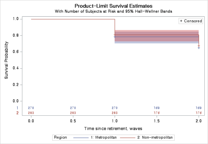
Survival analysis was used to examine transition to low AAI after retirement. The Cox risk set was defined among retirees with AAI ≥ 0.5 at the retirement wave. Time 0 was the retirement wave, the event was the first subsequent observation with AAI < 0.5, and censoring occurred at the last available follow-up without the event. Accordingly, 318 participants with AAI < 0.5 at the retirement wave and 1 participant with incomplete survival-time information were excluded from the Cox risk set, leaving 553 participants for the survival analysis.
$$\:h\left(t|X\right)={h}_{0}\left(t\right)\times\:\text{e}\text{x}\text{p}({\beta\:}_{1}Group+{\beta\:}_{2}Gender+{\beta\:}_{3}Age+\cdots\:+{\beta\:}_{p}{X}_{p})$$
Kaplan–Meier curves and log-rank tests were used to compare time to transition to low AAI between metropolitan and non-metropolitan retirees. Multivariable Cox proportional hazards models were then fitted to estimate the association between region of residence and transition to low AAI, adjusting for gender, age, education, marital status, smoking, drinking, and physical activity. Additional Cox models tested interactions between region and individual characteristics to assess whether predictors of transition to low AAI differed by region. The proportional hazards assumption was assessed using Schoenfeld residuals and showed no evidence of violation (p > 0.05). Because labor force participation was included in the AAI participation domain and could overlap conceptually with retirement status, we conducted a sensitivity analysis excluding labor force participation from the participation domain. Revised total AAI and revised participation-index models were estimated using the same piecewise GEE framework as the primary trajectory analysis. This analysis assessed whether the main regional trajectory findings and retirement-related changes persisted after removing the labor-force participation component from the AAI. All analyses were conducted using SAS version 9.4.