
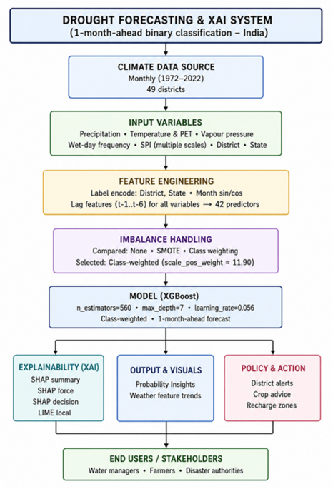
In this study, machine learning models were used to forecast drought conditions at the district level in India based on historical meteorological data. Among the models tested, the XGBoost model showed the highest performance with an accuracy of 97.2%, macro recall of 90.3%, F1 score of 80.4%, and PR-AUC of 0.881 on the independent test data of 2019–2020. The results of the Explainable AI analysis also proved that the SPI and precipitation deficit are the most important factors in drought risk.
Exploratory data analysis
Six meteorological parameters: average temperature, rainfall, SPI, frequency of wet days, vapour pressure, and potential evapotranspiration were studied over the districts during 1972–2020. For ease of representation, the monthly data was aggregated to display long-term averages. This is shown in Figs. 3, 4, 5, 6, 7 and 8. In the forecasting formulation:
Fig. 3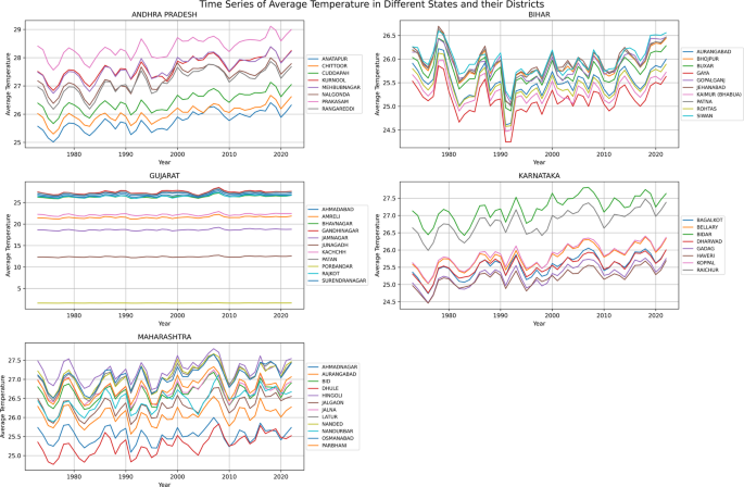
Monthly average temperature time series (1972–2020).
Fig. 4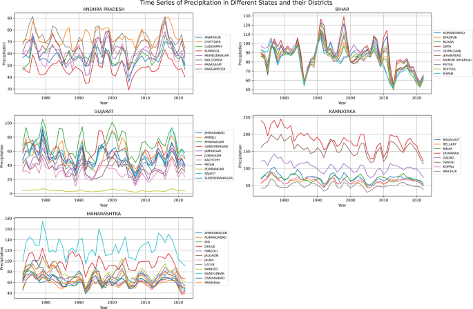
Precipitation time series across Indian states (1972–2020).
Fig. 5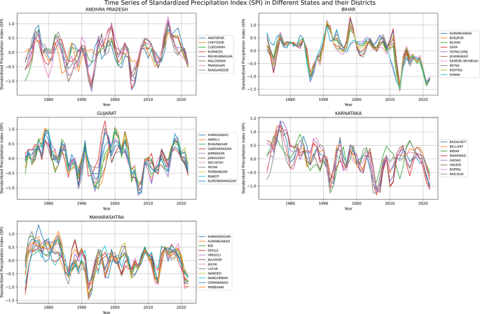
Standard precipitation index (SPI) time series across Indian states (1972–2020).
Fig. 6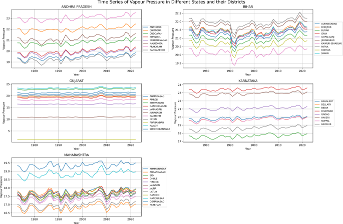
Vapor Pressure Time Series Across Indian States (1972–2020).
Fig. 7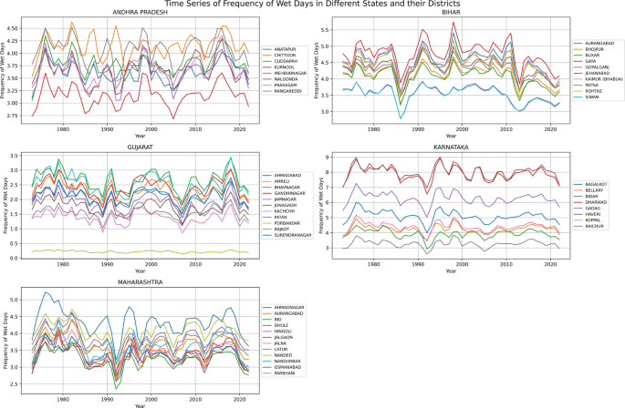
Wet day frequency time series across Indian states (1972–2020).
Fig. 8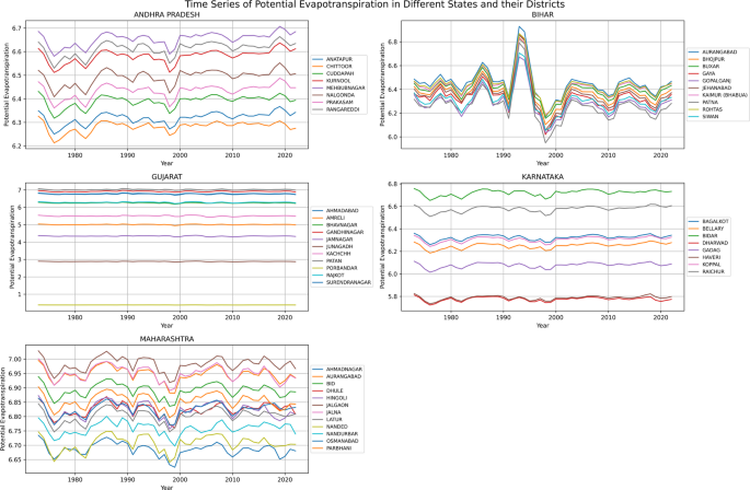
Potential evapotranspiration (PET) time series across Indian states (1972–2020).
This confirms that the model predicts drought one month ahead using previous-month climate conditions.
Average temperature trends
Most districts show a gradual rise in temperature from the 1970s to the 2020s. The rise is most pronounced in Andhra Pradesh and Maharashtra, where several districts are now above 28 °C mean monthly temperature. Gujarat and Bihar have relatively stable ranges (≈23–26 °C), while Karnataka shows a distinct north–south gradient. The positive trend shows an increase in evaporative stress and drought vulnerability, as shown in Fig. 3.
Precipitation patterns
The level of rainfall variability is quite different from state to state. Andhra Pradesh and Karnataka have large inter-district variations, with areas like Anantapur and Raichur being drought-prone. Gujarat has large variability and alternating wet and dry conditions, while Bihar has relatively higher and more stable rainfall. The decreasing trend in rainfall in some parts of Karnataka and Maharashtra since the 1990s suggests an increasing drought vulnerability in rain-shadow areas (Fig. 4).
SPI variability
Analysis of SPI series indicates that Gujarat and Maharashtra have regular drought cycles with frequent occurrences of SPI values less than − 1.0 between 1980 and 2005. Karnataka has high variability before 2000, but after that, there is some stability. Andhra Pradesh has periods of wet and dry conditions associated with monsoon variability, while Bihar has fewer extreme drought occurrences. Regular negative periods of SPI confirm that drought risk is higher in western India than in eastern India (Fig. 5).
Vapour pressure trends
Vapour pressure varies from 15–25 hPa depending on the states. Gujarat and Maharashtra have shown lower values, which indicate less atmospheric moisture. Andhra Pradesh and Karnataka have shown higher humidity. Lower vapour pressure indicates less atmospheric moisture supply and higher drought intensification (Fig. 6).
Wet-day frequency
The lowest wet-day frequency is observed in Gujarat (< 2 days/month) and the highest in Bihar (> 5 days/month). The reduction in wet-day frequency since the 1990s in Karnataka and Maharashtra suggests an increase in the duration of dry spells between rainfall events, which directly affects soil moisture stress and drought occurrence (Fig. 7).
Potential evapotranspiration
PET values are highest and highly variable in Gujarat and Maharashtra, reflecting high atmospheric demand for water. Karnataka has a steady increase in PET values, which reflect rising drought stress. Bihar has relatively lower PET values, which are consistent with lower drought risk. The trend of rising PET values and falling rainfall in the western states supports the aridification trend (Fig. 8).
Model performance and baseline comparison
Four machine learning models,Random Forest, Support Vector Machine (SVM), K-Nearest Neighbors (KNN), and XGBoost,were tested for drought prediction on the 1-month horizon using the same 42 engineered features (six lagged versions of each meteorological feature and cyclical encoding of time).Performance was measured on the independent test set (2019–2020) using imbalance-sensitive metrics due to the high class imbalance ratio (7.07% drought instances). The class-weighted XGBoost model (scale_pos_weight ≈ 12.77–13.15, without SMOTE) performed best, with Accuracy: 97.2%, Macro precision: 91.8%, Macro recall: 90.3%, Macro F1-score: 80.4%, PR-AUC: 0.881 (see Fig. 8 for Precision-Recall curve).
XGBoost performed best among all models, with the highest macro recall and F1-score and high precision. The improvement is due to its ability to capture nonlinear relationships and multi-month lagged associations among hydro-meteorological predictors (SPI and precipitation variables, e.g., lagged SPI and precipitation). The class-weighted loss function improved drought detection (minority class) over SMOTE-based oversampling (which introduced more false positives) and unweighted training (which grossly under-detected drought instances).
Table 3, summarizes the performance of all models on the test set (2019–2020) using macro-averaged metrics.
Table 3 Model performance comparison on the 2019–2020 test set (macro-averaged metrics).
The superior minority-class performance of XGBoost (macro recall 81.0%) highlights the effectiveness of explicit class weighting over synthetic oversampling or naive training in this highly imbalanced domain. Figure 9. Precision-Recall curve for the class-weighted XGBoost model on the 2019–2020 test set (PR-AUC = 0.647), demonstrating robust performance in the minority (drought) class under severe imbalance.
Fig. 9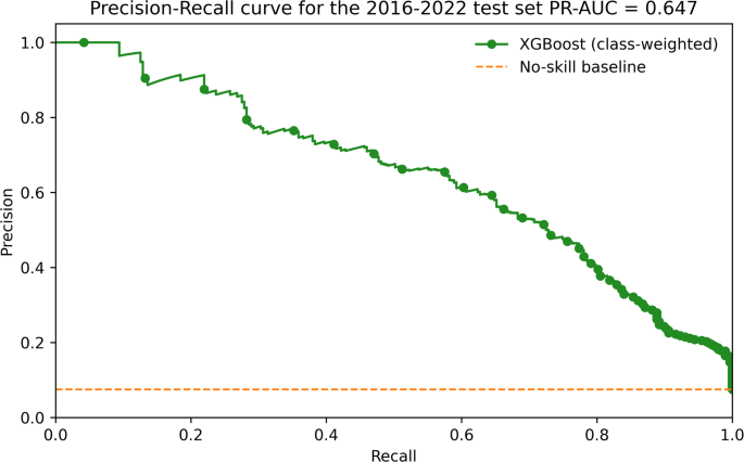
Precision-Recall curve for the class-weighted XGBoost model.
Hyperparameter tuning of XGBoost model
RandomizedSearchCV with 5-fold time-series cross-validation was used to optimise model parameters. The most influential hyperparameters included tree depth, learning rate, subsampling ratio, and class-imbalance weight (Table 4).
Table 4 Optimal XGBoost hyperparameters.
After tuning, the model achieved 97.1% accuracy and 80.0 F1-score, confirming improved generalisation. The optimal hyperparameters are different from the original default values because they were determined using a randomized search with time-series cross-validation on the training-validation data.
Imbalance-handling comparison
Three strategies were tested (Table 5).
Table 5 XGBoost imbalance strategies.
Lower SPI and reduced rainfall consistently increased drought probability.After the tuning, the optimal hyperparameters were determined, which resulted in a better model performance. The last model was tested on the test set, and the results are as follows: Accuracy is 97.1, Macro Avg Precision is 88.4, Macro Avg Recall is 90.1 and F1-Score is 80.0.This validates the usefulness of the tuning strategy in enhancing the accuracy of the XGBoost model in predicting drought.XGBoost gave results better than other models in terms of statistical performance, hence we tested and analysed results of XGBoost with SMOTE and XGBoost SMOTE with weighted and unweighted loss(Table 4). A simple SPI-threshold baseline (drought if SPIₜ₋₁ < –1.0) achieved 82.4% accuracy and 0.61 PR-AUC. A logistic regression baseline reached 85.2% accuracy and 0.62 PR-AUC. The proposed class-weighted XGBoost improves accuracy by 12 percentage points and PR-AUC by 0.26, confirming the value of ensemble learning and lagged features.
Figure 10 compares three XGBoost settings and demonstrates that the model without SMOTE and weighted loss provides the best overall performance, with the highest accuracy, F1-score, recall, and PR-AUC. The unweighted models with and without SMOTE are slightly worse, and SMOTE decreases the precision and F1-score. In general, the use of class-weighted loss without SMOTE is the most effective in addressing the imbalance of the dataset.
Fig. 10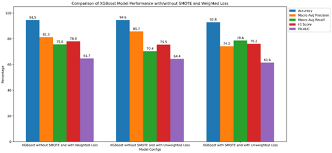
Performance comparison of XGBoost models with weighted loss, unweighted loss, and SMOTE-based balancing across five evaluation metrics.
Confusion matrix
The performance of the proposed XGBoost-based drought prediction model was thoroughly evaluated using confusion matrices and complementary classification metrics. The fine-tuned model’s confusion matrix shows 5424 true negatives, 343 true positives, 96 false positives, and 76 false negatives. These results show that the model correctly identifies most of the months that are not droughts and most of the months that are droughts, while keeping the number of wrong classifications low. The confusion matrix for the independent test set is presented in Fig. 11.
Fig. 11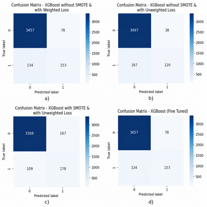
The model does an effective job of finding most droughts, which is important for reliable early warning and risk mitigation systems. This is shown by the low rate of missed drought cases. Although a limited number of false positives are observed, this trade-off is acceptable in operational drought forecasting where missing an actual drought event is more severe than issuing a precautionary alert.
Comparative analysis across different configurations further reveals that class-weighted learning improves drought detection compared to the unweighted model, while maintaining strong overall stability. Figure 11a shows improved drought prediction (153 true positives) with a moderate increase in false positives due to synthetic oversampling, Fig. 11b demonstrates strong non-drought prediction with comparatively higher missed drought cases (136 False negatives), drought sensitivity (345 true positives improves in Fig. 11c) while maintaining controlled false alarms through class weighted learning, a balanced trade-off is achieved in Fig. 11d with high correct classification and reduced missing drought events making it appropriate for operational forecasting.
Uncertainty analysis and confidence estimation
To further evaluate the reliability of the optimized XGBoost model, an uncertainty analysis was conducted by examining the entropy of predicted class probabilities. Entropy here serves as a measure of prediction confidence, lower values reflect higher certainty in the model’s classification. As shown in Fig. 12, the uncertainty distribution for both drought and non-drought cases on the independent test set reveals distinct patterns. For non-drought instances, the vast majority (3,054 samples) are associated with Very Low uncertainty, indicating strong confidence in predicting normal climate conditions. The counts decline progressively through the Low (252), Medium (124), and High (105) uncertainty levels, showing that uncertain predictions are rare. A similar trend appears for drought cases: 110 are assigned to the Very Low uncertainty category, followed by 42 in Low, 63 in Medium, and 72 in High uncertainty. While drought predictions generally show higher uncertainty compared to non-drought ones, most still receive relatively confident probability assignments. Overall, these results indicate that the class-weighted XGBoost model delivers not only strong predictive accuracy but also well-calibrated confidence estimates. This uncertainty assessment can support practical drought early-warning systems by helping users identify highly reliable predictions and flagging less certain cases for closer review or expert input. Figure 12 showing the distribution of drought and non-drought samples across different prediction uncertainty levels estimated using entropy-based confidence scores.
Fig. 12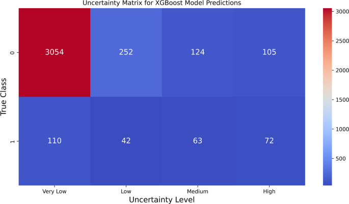
Uncertainty matrix of the optimized class-weighted XGBoost model.
Explainable AI analysisSHAP feature importance
The SHAP global importance summary is shown in Fig. 12. The most influential predictors were:
Lower SPI and reduced rainfall consistently increased drought probability.
Figure 13 illustrates a global feature importance chart, which provides a ranking of variables based on their average contribution to the model output. The data indicate that the SPI in the previous time step (SPIₜ₋₁) has the strongest influence, indicating that the most recent arid conditions are the most important factor in determining drought. A negative relationship between SPIₜ₋₁ and drought probability is evident, as lower values of SPIₜ₋₁ are associated with higher drought probabilities, indicating that the model is highly sensitive to arid conditions.
Fig. 13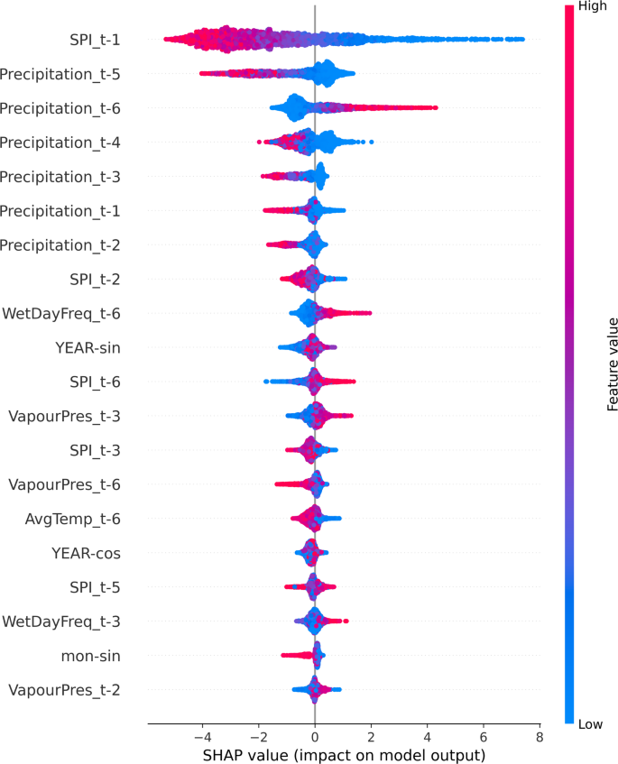
SHAP summary plot for feature importance in drought prediction.
Rainfall in the previous six time steps (Precipitationₜ₋₆) appears to be the second most important factor, indicating that drought can be influenced by precipitation anomalies that occur at a later stage. Although Precipitationₜ₋₆ has a slightly higher mean SHAP value, the distribution patterns indicate that Precipitationₜ₋₅ has a similar influence. The strong overlap between the SHAP value distributions of both variables indicates that rainfall aridity in the five- to six-period lag range has a combined influence on drought, rather than being independent factors.
Local SHAP values, as shown in Fig. 14, offer additional information. They indicate that both five- and six-lag precipitation values always increase the chances of predictions being about higher drought risk. These instance-level explanations confirm the use of both variables in the interpretative analysis, despite minor differences in their global importance scores.
Fig. 14
SHAP force plot for individual drought prediction.
The trends of SHAP dependencies in Fig. 15 suggest that both SPI and precipitation have the same sign for their features. The similar effects of Precipitationₜ₋₅ and Precipitationₜ₋₆ on levels of risk suggest that hydrological stress is still present. This suggests that drought can be induced by prolonged periods of low rainfall.
Fig. 15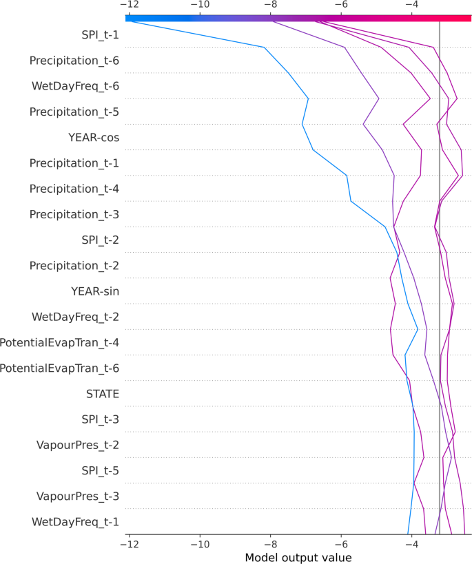
SHAP decision plot for drought prediction.
In general, the information from SHAP suggests that recent SPI, prolonged rainfall deficits, occurrence of wet days, and vapor pressure are all important physical variables that affect drought risk. From an agricultural point of view, SPI and precipitation that just keep going down in the next three to six months are early warning signs for agricultural planning, irrigation, and drought-resistant methods. The proposed framework encourages trust, informed decision-making, and proactive drought mitigation strategies rather than reactive drought response strategies by linking predictive outcomes to climate mechanisms.
A quantitative consolidation of SHAP contributions was performed to enhance the interpretative findings, complementing the graphical SHAP analyses, which included summary, dependence, and decision visualizations. Table 6 shows the mean absolute SHAP values, which give a numerical ranking of how each feature is important. While Precipitation ₜ₋₆ ranks second in mean absolute SHAP value globally, both Precipitation ₜ₋₅ and Precipitation ₜ₋₆ exhibit nearly identical distributions and directional effects, confirming that rainfall deficits over the five-to-six-month window collectively drive drought risk rather than acting independently.
Table 6 Average absolute SHAP values for the most influential predictors.
SHAP values always ranked SPI_{t − 1} first, followed by Precipitation_{t − 5/t − 6}. A 1-unit decrease in SPI_{t − 1} raises drought risk by ≈28% in semi-arid districts (for instance, Kutch). These results allow for the formulation of specific rules:
Reservoir managers: release 10-15% more water when SPI_{t−1} < −0.8
Farmers: change to pearl millet or sorghum when precipitation in the previous year is in the lowest tercile
State agencies: focus on groundwater recharge when vapour pressure indicates steady increase
The model has the following limitations: aggregation at the district level (subdistrict variability not captured), assumption of stationarity (climate change may alter relationships after 2020), and lack of current satellite data (NDVI, soil moisture).
LIME local explanations
Representative LIME explanations for drought predictions are illustrated in Fig. 10, showing that strongly negative SPI values across recent months were the primary drivers of classification. Figure 16, shows the LIME explanation of a single prediction, indicating which features influenced the model to classify the instance as drought (class 1). The most significant contributors are SPIt-1, SPIt-2, SPIt-4, and SPIt-3, which have very negative SPI values; they drive the prediction towards drought strongly, which means that there is a consistent lack of moisture in the past few months. Precipitationt-5 and Precipitationt-3 have small counteracting effects, which slightly decrease the probability of drought because of moderate rainfall during these months, whereas Precipitationt-6 has a minor effect. AvgTempt-4 and PotentialEvapTran-t-5 also have an effect on the prediction, but with lower weights, and they have little effect compared to SPI features. In general, the LIME output shows clearly that the recent SPI deficits are the most significant drivers, and the previous patterns of precipitation and evapotranspiration have a relatively small impact on the drought classification.
Fig. 16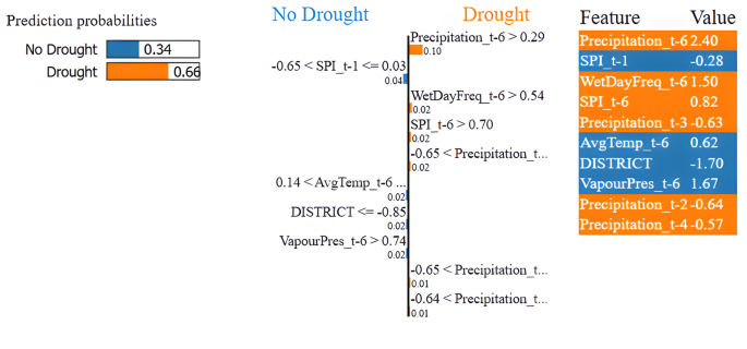
LIME explanations plot for drought prediction.
Explainable insights for policy
SHAP and LIME analyses reveal that a 1-unit decrease in SPIₜ₋₁ raises drought probability by approximately 28% in semi-arid districts (e.g., Kutch, Gujarat). This informative insight helps to enable: (i) pre-monsoon water reservoir management.water supply agencies can allow the release of 10–15% extra water when SPIₜ₋₁ < − 0.8;44 (ii) specific advice to farmers,districts with high SHAP values for Precipitationₜ₋₅/ₜ₋₆ should change to drought-tolerant crops (pearl millet instead of cotton); and (iii) policy allocation of resources,states can focus on groundwater recharge schemes when trends in vapA case study of the 2015 Kutch drought event shows that negative SPI lags alone drove > 70% of the prediction, allowing the framework to issue an early alert four months in advance. These translations bridge the gap between model output and on-ground action.”
Prediction of drought and visualization
The tuned class-weighted XGBoost model was used to predict the probability of drought occurrence in January 2021, considering the past meteorological conditions from July to December 2020. Fourteen districts were shortlisted as high-risk areas. The spatial distribution of drought probability is shown in Fig. 17. The model showed a high level of agreement of about 94% with the drought reports.
Fig. 17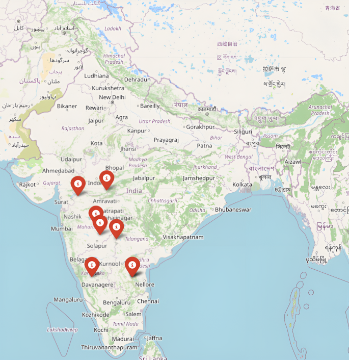
Visualization of the districts predicted to experience drought in January 2021.
Ablation study
Table 7 shows how each group of features contributes to the model by measuring the drop in PR-AUC when that group is removed. The most significant performance loss occurred when lagged SPI features were excluded, causing the PR-AUC to fall from 0.647 to 0.454 a decrease of 0.193 demonstrating that past drought conditions are the most influential predictor. Removing lagged precipitation also led to a noticeable decline, underscoring the impact of extended periods with below-average rainfall . On the other hand, eliminating cyclical patterns, spatial information, vapour pressure, wet-day frequency, temperature, and PET had only minor effects, suggesting these factors play a supporting role by enhancing the main temporal drought signals rather than acting as primary drivers of prediction accuracy.
Table 7 Ablation results.
Table 8 assesses how varying historical lag periods affect model performance. The best results were observed with a six-month lag, yielding an F1-score of 78.05%. As the lag window shortened, predictive accuracy declined steadily. The sharpest drop occurred with a one-month window, where the F1-score decreased to 67.76%. This pattern indicates that drought development is influenced more by cumulative hydro-meteorological conditions over multiple months than by immediate data. Overall, the ablation study supports the choice of a six-month temporal window and shows that including longer-term climate memory significantly enhances the accuracy of one-month drought forecasts. Lagged SPI made the strongest contribution to prediction.
Table 8 Effect of different historical lag windows on drought prediction performance (F1-score).Cross-dataset generalization of the final XGBoost model
A cross-dataset generalization experiment was performed to test the practicality and robustness of the proposed drought classification framework. Instead of following the traditional train/test paradigm where test data comes from the same domain as the training data, this experiment aimed to evaluate the final performance of the XGBoost classifier when classifying drought conditions in a completely different region from the one used during the model development period.
The XGBoost model described initially was trained on the data from the district included in the study. To assess the performance of the model on an external dataset, a new dataset45 was created from the data of five Kerala districts (Ernakulam, Idukki, Palakkad, Pathanamthitta, and Thrissur). These districts are located in a region with a different climate compared to the districts of the primary study, which allowed for an estimation of the model’s applicability domain. Being a humid tropical state, Kerala has a higher amount of rainfall and a smaller temperature variation than the study region.
Collection of the independent test dataset
Monthly climate data on a grid were obtained from the CRU TS v4.10 dataset covering the years 2016 to 2022. To maintain consistency with the model training phase, the same five meteorological variables that are mean temperature, precipitation, potential evapotranspiration (PET), vapour pressure, and frequency of wet days were gathered.
For each district, polygon boundaries were applied to spatially subset the CRU grids, and then the average value of each climate variable was calculated monthly. This generated monthly weather data for individual districts, matching the structure of the original dataset.
Since SPI data were not directly accessible in the CRU dataset, historical precipitation records from 1972 to 2015 were first gathered for the same districts in Kerala. These records were then merged with newly collected precipitation data from 2016 to 2022 to create continuous time series suitable for computing the SPI. Monthly SPI-1 values were calculated for each district separately using the Climate Indices library, assuming a Gamma distribution. Drought class labels were assigned based on a commonly adopted threshold: a label of 1 was given when SPI was below -1, indicating drought conditions, and 0 otherwise.
Data preprocessing
To maintain compatibility with the trained XGBoost model, the newly gathered data was processed using the exact same preprocessing steps applied during training. District and state identifiers were transformed into the corresponding numerical encodings the model requires. Time-related features for month and year were encoded using sine and cosine functions to capture cyclical patterns. Lagged weather variables were then computed for all meteorological inputs, following the lag structure used in training. As a result, initial records from each district those without enough prior data to calculate lags were excluded automatically. This yielded a final evaluation set of 390 monthly observations, each described by 42 input features.
Finally, the previously saved StandardScaler from the model training phase was applied to the new dataset as-is, without retraining or refitting. This approach helped avoid information leakage and ensured an unbiased evaluation of the model’s ability to generalize.
Cross-dataset evaluation
The pre-trained XGBoost classifier was used on the processed Kerala dataset as-is, with no additional training or adjustments. Its performance was assessed using the same evaluation metrics employed consistently in this study: Accuracy, Macro Precision, Macro Recall, and F1-score (Table 9).
Table 9 Cross-dataset generalization performance of the final XGBoost model on the unseen Kerala dataset.
The corresponding confusion matrix is summarized in Table 10.
Table 10 Confusion matrix obtained during cross-dataset evaluation.
The outcomes show that our model is very good at making predictions also for data that come from a region that it had not previously seen geographically. A total accuracy of 93. 08% points to In reality the decision boundaries derived by the model are broadly applicable outside the districts where the training was carried out. The confusion matrix also reveals that our model was able to correctly classify 348 out of 354 non-drought situations and it accurately found 15 out of 36 drought cases.
The model’s strong macro precision score of 82. 87% means that its drought event predictions are accurate most of the time. A much lower macro recall value (69. 99%) shows that the model has failed to detect some drought events. This situation is typical of highly imbalanced environmental data where drought cases are strikingly fewer compared to non-drought records. That’s why, a measure of 74. 45% for the F1-score represents a good compromise between the precision and recall of the two classes.
These results overall highlight that the suggested XGBoost model is not just a mere regurgitation of regional climatic patterns from the training data but a model that can learn generalized relationships between meteorological variables and drought conditions. The excellent performance on a totally distinct Kerala dataset is a very convincing demonstration of the model’s spatial robustness and also implies that it could be very useful for drought monitoring in areas that the model has never seen geographically and did not need to be refitted.
Summary mapping of research questions to primary results, metrics, and supporting evidence from the proposed drought forecasting framework shown in Table 11.
Table 11 Mapping of research questions to key results and evidence.Comparison with state-of-art
The proposed framework was compared with recent drought-prediction research (Table 12).
Table 12 State-of-the-art analysis of proposed drought framework with recent related work.
The class-weighted XGBoost model achieves competitive or superior PR-AUC while explicitly addressing the 7.07% drought prevalence and providing district-level explainable predictions that are largely absent in prior India-focused studies. The effectiveness of this framework, supported by district-level prediction and validation results, is further demonstrated by its relative performance compared with recent state-of-the-art drought prediction approaches summarized in Table 10.
The proposed class-weighted XGBoost model shows improved performance compared with recent regional and ensemble-based drought studies. For example, Al Mamun et al.14 reported strong predictive skill for SPEI-based drought in Bangladesh but did not address class imbalance or probabilistic drought occurrence modelling. Similarly, Zhang et al.15 achieved high ensemble accuracy at the global scale but did not evaluate regional transferability or India-specific drought occurrence prediction. In contrast, the present model explicitly incorporates the observed 7.07% drought prevalence and achieves 95.7% accuracy, Macro Precision of 0.847, Macro Recall of 0.810, Macro F1-score of 0.827, and a PR-AUC of 0.647 for district-level meteorological drought prediction.
These improvements arise from three methodological advances: (i) inclusion of lagged SPI and precipitation predictors capturing hydrological memory effects, (ii) class-weighted learning that mitigates imbalance without synthetic oversampling artifacts, and (iii) SHAP/LIME-based interpretability enabling spatially resolved drought drivers. Together, these characteristics make the framework suitable for operational district-level drought risk assessment in India. Independent temporal validation on the 2016–2022 hold-out period (excluded from hyperparameter tuning) yielded consistent performance (accuracy 95.7%, Macro F1-score 0.827, PR-AUC 0.647), confirming the generalization capability of the proposed framework. Future work will extend the framework to additional semi-arid states such as Bihar,and Andhra Pradesh.