
Description of the study area
The Mitidja Plain, located in north-central Algeria between 36°30’ and 36°45’N and 2°30’ and 3°00’E, covers an area of about 2561 hectares (ha)35 and is bordered by the Mediterranean Sea to the north and the Tell Atlas Mountains to the south, as shown in Fig. 1. It is characterized by fertile Quaternary alluvial deposits36,37, a Mediterranean climate with 600–800 mm annual rainfall38, and extensive agricultural activity including cereals, fruits, and vegetables. Despite its importance as one of Algeria’s most productive agricultural regions, the plain faces severe soil erosion risks due to steep slopes, intensive land use, and rainfall variability39.
Fig. 1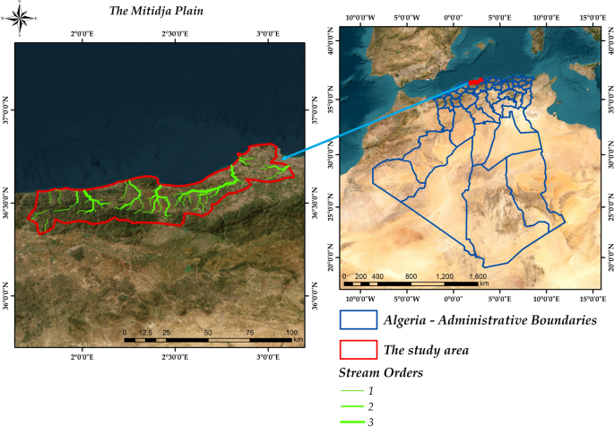
Location map of the study area (Generated by ArcGIS 10.2.2. software; Esri (Environmental Systems Research Institute, Redlands, CA, USA; https://support.esri.com/en-us/patches-updates/2016/arcgis-10-2-2-for-desktop-engine-server-update-geopacka-2093).
The study methodology
The GEE-based approach delivered a comprehensive spatial analysis of large-scale geospatial data for soil erosion risk across the Mitidja plain, combined with the AHP technique that was applied to analyze different environmental parameters and involves ranking based on certain criteria to solve a very complex decision-making process were used to estimate average soil loss (\(\:A\)) using the RUSLE equation. This equation is calculated using specific factors for the study area, including rainfall-runoff erosivity (RE), soil erodibility (KS), slope length steepness (LS), cropping management (CM) and management practices (PC), these factors represent the specific environmental and land-use conditions that contribute to the overall soil erosion hazard assessment over the investigated area. This study methodology was outlined in the following flowchart (Fig. 2).
Fig. 2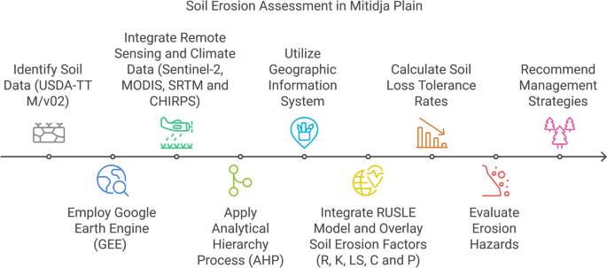
The study methodological framework.
The data Preparation and processing
In this study, data from the Sentinel-2, Multispectral Instrument (MSI) Level-1 C (COPERNICUS/S2_SR), provided by the European Space Agency (ESA, http://www.esa.int/Our_Activities/Observing_the_Earth/Copernicus/Overview4), and the MODIS sensor onboard NASA’s Terra and Aqua satellites (http://search.earthdata.nasa.gov/search) were utilized, accessed on 16 May 2024. Sentinel-2 offers wide-swath, high-resolution (10 m) multispectral images that support land monitoring for applications such as vegetation, land use/land cover assessment, and the observation of inland and coastal water bodies40. MODIS data, known for its wide spectral range and cost-effectiveness, is frequently used for monitoring vegetation health and surface conditions and it is particularly useful for studying soil erosion due to its timely availability and ability to provide frequent, medium-resolution data41. MODIS images undergo several corrections such as radiometric, geometric, and atmospheric to ensure their accuracy. In this study, MODIS/061/MCD12Q1 data with an 8-day time resolution and 500 m spatial resolution were employed to calculate soil erosion; cropping management and supporting conservation practices factors (30 m) using the GEE platform based on AHP technique.
The key variables used in this soil erosion study include: (a) annual rainfall data obtained from the Climate Hazard Group Infrared Precipitation with Station Data (CHIRPS) (0.05°, approximately 5 km) database (https://chc.ucsb.edu/data/chirps), which was used to calculate the rainfall runoff erosivity factor (30 m)42, (b) slope length and steepness factors derived from the Shuttle Radar Topography Mission (SRTM, USGS/SRTMGL1_003) digital elevation data with a resolution of 1 arc-second (approximately 30 m), available on a near-global scale (https://earthexplorer.usgs.gov/), (c) land use and normalized difference vegetation index (NDVI) determined from Sentinel-2 imagery, and (d) soil type and characteristics collected from (USDA-TT M/v02) soil texture classes at six different soil depths (0, 10, 30, 60, 100, and 200 cm) with a resolution of 250 m (https://websoilsurvey.nrcs.usda.gov/app/).
Additionally, ArcGIS 10.2.2 software was used to create maps illustrating location map of the study area, soil erosion factors thematic maps, annual soil loss (RUSLE model) map and soil erosion potential hazards map.
Soil erosion thematic maps computation: RUSLE model
To estimate, predict, quantify, and assess the annual average soil loss rate the average annual soil loss per unit area (\(\:A\), t ha−1 yr−1) for a given area under particular management conditions, and estimate the soil erosion process spatial mapping using GEE-based approach, the RUSLE was utilized as widely used soil erosion empirical-based model, relies on various factors such as rainfall-runoff erosivity (RE MJ mm ha−1 h−1 yr−1), soil erodibility (KS t ha MJ−1 mm−1), slope-length (L) and slope-steepness (S) factors (LS), cover and management (CM), and conservation practices (CP), as numerical representation of the particular conditions that influence the soil erosion risk in the region under study, and the LS, CM, and CP factors are dimension less values.
According to Renard, 199743, the RUSLE model was used in the current study for soil erosion assessment through the following Eq. 1:
$$\:A={R}^{E}\times\:{K}^{S}\times\:{L}^{S}\times\:{C}^{M}\times\:{C}^{P}$$
(1)
Based on McKague, 202344, soil erosion values and tolerance rates are closely linked to both soil characteristics and management practices, as shown in Tables (1 and 2).
Table 1 Soil erosion factors and management strategies to reduce soil losses.Table 2 Soil erosion classes and soil loss tolerance rates.Rainfall-runoff erosivity factor (RE)
Based on GEE-based approach, the rainfall-runoff erosivity RE factor plays a crucial role in influencing potential sheet and rill soil erosion and quantifies soil erosivity based on the aggressiveness of daily basis runoff sediment deposits in the study area over a given time period (2001–2023)45, and it was considered as a major challenging task due to unavailability of high-resolution rainfall-runoff database for the investigated area. The RE factor was calculated using the linear relationship empirical Eq. 2, that was developed by Choudhury and Nayak, 200346.
$$\:{R}^{E}=79+\left(0.363\text{*}{X}_{a}\right))+89.7$$
(2)
where RE is the rainfall-runoff erosivity factor and Xa is the annual precipitation average (mm).
The soil erodibility factor (KS)
The KS factor is one of the most significant barriers for soil erosion modeling on large spatial scales is insufficient data on soil attributes47. KS factor describes the predisposition of soil particles to be transported and separated by runoff and plays a crucial role in evaluating the inherent vulnerability of soil to erosion caused by rainwater and runoff48.
The KS factor is rated primarily on a scale of 0 to 1, with higher values indicating a greater susceptibility to soil erosion, relies on various soil characteristics encompassing mineralogical, physical, chemical, and morphological features such as soil texture classes, soil structure, organic matter content, soil permeability, and infiltration.
In this study of the Mitidja plain, we employed CBG analysis using GEE platform to estimate the KS factor, utilized soil types and texture maps to conduct geospatial analyses efficiently, providing a robust and scalable approach. This approach considers local variations and characteristics, accurately representing soil erosion factors within the study area.
The KS factor was calculated by means of the following Eqs. 3 and 4, which were developed from global data of measured KS values by Renard, 199743:
$$\:{K}^{S}=0.0034+0.0405\:\text{x}\text{exp}\left[-0.5\:{\left(\frac{{log}{D}_{g}+1.659}{0.7101}\right)}^{2}\right]$$
(3)
$$\:{D}_{g}=\text{exp}\left(\sum\:{f}_{i}\:In\:\left(\frac{{d}_{i}+{d}_{i-1}}{2}\right)\right)$$
(4)
where Dg is the particle size geometric mean, for clay, silt, sand texture classes, di is particle size maximum diameter (mm), di−1 is particle size minimum diameter, and fi is the mass fractions.
McKague, 202344 clarified the KS factor rates for various soil textures corresponding to organic matter content, as represented in Table 3.
Table 3 Soil texture and corresponding soil erodibility factor rates.Topographic (slope-length (L) and slope steepness (S) factors (LS))
The LS factor in RUSLE is a crucial component in assessing soil erosion rates and expressed as the ratio extracted from the SRTM satellite data, integrates slope length (L) and slope steepness (S) into a unified index by considering the distance from the runoff initiation point to the deposition area using GEE, CBG analysis computation49. LS factor reflects the influence of topography on soil erosion, standardized at a length of 22.1 m and a steepness of 9%, demonstrated that increases in slope length and slope steepness with the greatest accumulation can produce higher overland flow velocities, increases transport detachment and capacity with correspondingly higher erosion50.
The LS factor was defined by Shinde et al., 201151 and expressed as the following Eq. 5.
$$\:{L}^{S}={\left(\frac{L}{22.1}\right)}^{\:}\text{*}\left(65.4\text{*}\left({sin}\theta\:\right){\:}^{2}+4.56\text{*}{sin}\theta\:+0.0065\right)$$
(5)
where L is the slope length (m), and S is the slope gradient (%).
The LS factor rates were clarified for various topographic factors by McKague, 202344, shown in Table 4.
Table 4 Slope length and slope steepness data and corresponding LS factor rates.Crop cover and management factor (CM)
The Crop cover and management factor CM is used to determine the impacts of cropping and management practices in agricultural management and is notably susceptible to human influence to mitigate soil erosion52. Sentinel-2 data from Google Earth Engine (GEE) were employed to address land cover data based on the maximum likelihood algorithm and ground truth verification points. This approach leverages the geospatial cloud-based analysis capabilities, offering a more efficient method for land cover and management in the Mitidja plain that is very sensitive to potential tilled soil erosion under Mediterranean conditions to the consequent loss from continuous fallow land. the CM factor together with LS factor is most sensitive to soil loss. In this study, the CM factor was evaluated through the most widely used satellite derived normalized difference vegetation index (NDVI) indicator, as an indicator of the energy reflected by the earth related to various cover type conditions following the empirical Eqs. 6 and 753.
$$\:{C}^{M}=\text{exp}[\alpha\:\frac{NDVI}{(\beta\:-NDVI)}]$$
(6)
$$\:NDVI=\frac{NIR-R}{NIR+R}$$
(7)
where CM is the crop cover and management factor; α and β are the parameters that determine the shape of the curve relating to NDVI; NIR is near infrared band and R is red band.
The CM factor rates for crop management values of the present study ranging from 0 to 1, where a lower CM suggests minimal soil loss that was assigned to a few pixels with negative values, and the maximum value indicates higher susceptibility to soil loss that was assigned to pixels with value greater than 1, as explained by McKague, 202344 and shown in Tables 5 and 6.
Table 5 Crop cover and management factor (CM) rates.Table 6 Tillage method (CM factor) rates.Conservation practice factor (CP)
The CP factor represents the effectiveness of management practices and soil loss ratio of up-and down-slope tillage through vegetation caver, soil biomass, and runoff control, as determined by agronomical practices54. The CP factor was calculated using remote sensing-driven analyses methodology in GEE-based approach based on Sentinel-2 image by defining a function that extracts relevant bands or properties for conservation practice, allowing for a comprehensive assessment of soil erosion susceptibility43.
The CP factor rates for conservation support practices, as represented by McKague, 202344, are shown in Table 7.
Table 7 Conservation practice factor CP rates.Multi-criteria decision using analytical hierarchy process (AHP)
AHP technique is a multi-criteria decision analysis method which applied in this study by integrating multiple factors and involves ranking based on certain criteria to solve a very complex decision-making problems, based on its interdependency and interrelationship between other parameter, and hierarchy model was done through higher to the lower level using a pairwise comparison of a different parameter which influences the soil erosion process expressed in a numerical scale and consistency ratio30,55, as represented in the following Eqs. 8 and 9:
$$\:M=\left[\:\begin{array}{cc}1&\:{a}_{12}\:\:\:\:\\\:{a}_{21}&\:1\\\:\begin{array}{c}{a}_{31}\\\:\vdots\\\:{a}_{n1}\end{array}&\:\begin{array}{c}{a}_{32}\\\:\vdots\\\:{a}_{n2}\end{array}\end{array}\begin{array}{cc}{a}_{13}\:\:\:\cdots\:&\:{a}_{1n}\\\:{a}_{22}\:\:\:\dots\:&\:{a}_{2n}\\\:\begin{array}{c}1\:\:\:\:\:\:\dots\:\\\:\vdots\\\:\dots\:\:\:\:\:\:\:\:\dots\:\end{array}&\:\begin{array}{c}\dots\:\\\:\vdots\\\:1\end{array}\end{array}\right]$$
(8)
where
$$\:{a}_{ij}=\frac{Weight\:of\:attribute\:i}{Weight\:of\:attribute\:j}$$
(9)
where a is the weight may vary in the numerical scale of 1 and 9 and the element of 1/1 in the matrix have equal importance for both parameters i and j based on a preference scale (SN) that represented in Table 8.
Table 8 Scale of preference for the analytical hierarchy process (AHP) pairwise comparison by Saaty, 198929.
The present study considered six individual parameters such as soil texture, OMC, slope, crop cover, tillage method, and support practice of the study area that have significant influence on the soil erosion. The highest eigenvalue of the matrix λmax for each factor was determined and computed by adding each column values of pairwise comparison matrix30.
The consistency of the pairwise comparison matrix of order n was calculated through the consistency index (CI) and consistency ratio (CR) that should be less than or equal to 0.1 to be accepted as consistent56, as represented in the following Eqs. 10 and 11:
$$\:CI=\frac{{\lambda\:}_{max}-n}{n-1}$$
(10)
$$\:CR=\frac{CI}{RI}$$
(11)
where RI is the average of resultant consistency index of randomly generated comparison and it varies according to order of the matrix30. The CR >0.1 endorses the omission of variable and CR <0.1 will allow the variables in the analysis.
When conducting comparisons, a compatibility ratio of 0.1 or lower signifies compatibility. Following this, a map depicting soil erosion was generated using CBG analysis in GEE platform based on the next specified Eq. 12:
$$\:A={(R}^{E}\times\:{\text{W}}_{i})\times\:{(K}^{S}\times\:{\text{W}}_{i})\times\:{(L}^{S}\times\:{\text{W}}_{i})\times\:({C}^{M}\times\:{\text{W}}_{i})\times\:({C}^{P}\times\:{W}_{i})$$
(12)
where Wi is the weight of each soil erosion factor.