Integrated in vivo combinatorial functional genomics and spatial transcriptomics of tumours to decode genotype-to-phenotype relationships

Animal experiments

Group size was determined on the basis of our experience in previous experiments68,69. For HDTV injections, eight-week-old female C57Bl/6 animals were purchased from Envigo. The mice were injected (into the lateral tail vein in 5–7 s) with 5 μg DNA of each of a total of eight perturbation plasmids (40 µg total DNA) mixed with 20 µg CMV-SB13 transposase (1:2 ratio) prepared in sterile 0.9% sodium chloride solution in a total volume corresponding to 10% of the body weight, as described before. Two animals were used. We labelled this approach RUBIX as the perturbation plasmids are equipped with molecular barcodes (Extended Data Fig. 1) and the plasmid mixtures injected allow for all possible combinations to become integrated in the genome of hepatocytes (Fig. 1a). All animals were monitored twice weekly and animal experiments were performed in compliance with all relevant ethical regulations determined in the animal permit. After tumours were palpable (10 weeks), the animals were euthanized and their livers were harvested (Extended Data Fig. 2). As a control group, two animals were injected with 40 µg pT3-EF1-shRen and 20 µg CMV-SB13 transposase (1:2 ratio) prepared in sterile 0.9% sodium chloride. For fixation, livers were incubated in 4% paraformaldehyde for 48 h. The sample processing procedure is illustrated in Extended Data Fig. 4. For the leave-one-out experiments (Fig. 7), HDTV injections were performed essentially as described before. For omission of either VEGFA or mtCTNNB1 perturbation from the plasmid pools, the respective plasmids were replaced with a control plasmid. Housing conditions for the mice were: 12 h light–12 h dark cycle, an ambient temperature of 20–24 °C and relative humidity of 45–65%. All animal experiments were approved by the regional board Karlsruhe, Germany.

10X Visium for FFPE spatial transcriptomics

Spatial transcriptomics were performed using the manual 10X Visium workflow for samples embedded in paraffin blocks or the 10X Visium CytAssist workflow for samples already placed on glass slides and stained with H&E (Extended Data Fig. 2). Both workflows were carried out according to the manufacturer’s protocol (CytAssist, CG000495, RevC; manual Visium, CG000407, RevD). Briefly, slices of approximately 5 µm were cut from FFPE blocks using a microtome and floated onto a water bath at 42 °C until all wrinkles were resolved. For the manual Visium workflow the slice was then placed inside the capture frame of the spatial transcriptomics slide (M.R.). Slices used for the CytAssist workflow were placed on frosted glass slides. Deparaffinization and staining of the slides was similar between both workflows. After drying the slide, paraffin was removed through incubation at 60 °C for 2 h and a subsequent incubation in xylol. Rehydration was done by sequential washes with decreasing ethanol concentrations. After rehydration, the tissue was stained with H&E and imaged using a Leica Aperio AT2 microscope at ×40 magnification. Following imaging, the slides were destained by incubation in 0.1 N HCl and formalin crosslinks were removed by incubation with TE buffer pH 9.0 for 1 h at 70 °C (manual workflow) or decrosslinking buffer for 1 h at 95 °C (CytAssist workflow.) The tissue was then permeabilized and incubated with RTL probes at 50 °C for approximately 20 h. Free probes were washed away and the bound probes were ligated, followed by washing steps to remove unligated probes. For the manual workflow, the probes were released by treating the slices with RNase and a permeabilization enzyme. For the CytAssist workflow, the slices were stained with a diluted eosin solution and placed in the CytAssist together with the Visium spatial transcriptomics slides and incubated for 30 min at 37 °C with RNase and permeabilization enzyme. For both protocols, the spatial barcode was added to the probes by extending them and the probes were released using a 0.08 M potassium hydroxide solution. For the CytAssist workflow, a pre-amplification PCR consisting of eight cycles was performed. After clean-up with 1.2× SPRIselect beads, 25% of the product was used as input for the index PCR. For both protocols, a quantitative PCR was used to select the number of cycles for the index PCR. To reduce PCR duplicates and avoid overamplification, cycle number at a Cq value of 10% was used for the index PCR. The PCR product was purified using 0.85× SPRIselect beads.

For samples already stained and mounted on a slide, the slides were first imaged and then incubated in xylol to remove the coverslip. Sample rehydration was done by sequential washes with decreasing ethanol concentrations. The slides were destained and decrosslinking was performed by incubating with a decrosslinking buffer at 95 °C for 1 h. After decrosslinking, the samples were incubated with probes for 20 h at 50 °C. Excess probes were washed away and the probes were ligated. Thereafter, the unligated probes were washed away. The samples were stained again with eosin and placed in the 10X CytAssist together with the spatial transcriptomics slides. A mixture of RNase and permeabilization enzyme was added to the spatial transcriptomics slides and the 10X CytAssist was started. After incubation, the spatial transcriptomics slides were removed and the enzymes were washed off. The spatial barcodes were attached to the probes with an extension enzyme. Probes were released using 0.08 M potassium hydroxide solution. The probes were then amplified through eight PCR cycles; 25% of the purified PCR products were used as input for the index PCR. The cycle number of the index PCR was determined using the cycle number at a Cq value of 10%.

For all samples, the final sample concentration was determined using Agilent Tapestation 4150 with D1000 HS tapes. Sequencing for both protocols was performed on an Illumina NovaSeq6000 system. Four samples were pooled on one SP flow cell with 100 cycles to aim for a read count of 250 × 106 reads per sample. The FASTQ files and the alignment were done using spaceranger 2.0.1. A total of 12 spatial transcriptomics datasets were generated (Extended Data Fig. 2). Note that the utility of sample ML-II_B_2Cyt is constrained by tissue detachment of the sample during the processing for 10X Visium CytAssist.

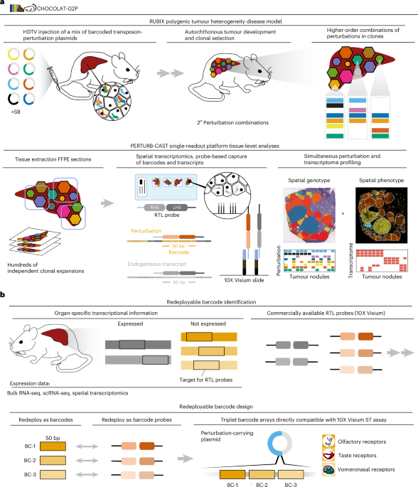
The 10X Visium for FFPE protocol engages RTL probes that capture a 50-nt sequence specific to endogenous transcripts (note that we used Visium mouse transcriptome probe set v1). We leveraged this strategy to likewise capture molecular barcodes via RTL probes (Fig. 1). We hence labelled this approach PERTURB-CAST.

Economized molecular barcode selection

To enable PERTURB-CAST, we aimed to avoid additional expenses and protocol modifications by redeploying RTL probes from commercially available 10X Visium reagents (originally designed to detect endogenous transcripts) as barcode identification reagents, provided that the selected transcripts are not expressed in mouse liver. We named this strategy redeploy probes for barcode capture (REDPRO-BC; Fig. 1 and Supplementary Fig. 1). To this end, we initially analysed a publicly available bulk RNA-seq dataset including a total of 128 murine liver samples (GSE137385)70 to identify transcripts that were generally not detected (fragments per kilobase of transcript per million mapped reads = 0 over all samples). Note that this approach can be error-prone due to the initial source data. Consequently, we went on to validate non-expression of selected transcripts (olfactory, vomeronasal and taste receptors) in additional datasets (including bulk RNA-seq from GSE148379)19, information provided in MGI GXD71 as well as 10X Visium data24. The endogenous transcripts associated with the REDPRO-BCs used in this study are illustrated in Extended Data Fig. 3 and the respective nucleotide sequences for 10X Visium RTL-probe capture barcodes (reverse complement to RTL-probe sequence provided by 10X Genomics) are listed under the section ‘Molecular cloning’. Note that we used Visium mouse transcriptome probe set v1. Visium mouse transcriptome probe set v2 is not compatible with the barcodes employed in this study.

Molecular cloning

The transposon plasmids used in this study including overexpression constructs for NICD, mutant human CTNNB1 (T41A) and human MYC and potent shRNA constructs targeting Trp53, Pten, Kmt2c and Renilla luciferase were previously described and validated in animal experiments19,68,72. For spatial transcriptomics, note that NICD overexpression can be investigated via Notch1 expression given that the 10X Visium RTL probe identifies the exogenous transcript introduced. However, endogenous Notch1 is similarly identified. VEGFA overexpression plasmid was cloned by insertion of a codon-optimized gene fragment (gBlock, IDT) based on Vegfa NCBI reference sequence NP_033531.3 by replacing hMYC from a previously validated expression plasmid68 using NEBuilder HiFi-DNA assembly according to the manufacturer’s protocol (NEB). All plasmids were individually modified to express molecular barcodes. Specifically, fluorescent protein-based peptide barcodes (mKate2, mOrange2 and mWasabi) were ordered as codon-optimized gene fragments (gBlock, IDT) and cloned into previously validated shRNA expression plasmids to replace GFP68 using NEBuilder HiFi-DNA assembly according to the manufacturer’s protocol. Small-peptide barcodes (for example, AU1, AU5 and so on), as described previously14, were ordered as oligonucleotides (Sigma), annealed and cloned using NEBuilder HiFi-DNA assembly according to the manufacturer’s protocol. Long RNA barcodes (stretches of at least 650 nt derived from the combination of multiple oligonucleotide–miner probe sequences designed against Arabidopsis thaliana Chr1 (ref. 73) were ordered as gene fragments (gBlock, IDT) and cloned using NEBuilder HiFi-DNA assembly according to the manufacturer’s protocol. REDPRO-BC triplet arrays were ordered as gene fragments (gBlock, IDT) and cloned using NEBuilder HiFi-DNA assembly according to the manufacturer’s protocol. Briefly, each REDPRO-BC triplet array incorporates one 50 nt sequence derived from olfactory receptors, one 50 nt sequence derived from taste receptors and one 50 nt sequence derived from vomeronasal receptors (based on 10X Genomics RTL-probe sequences against murine transcripts; note that we used Visium mouse transcriptome probe set v1; sequences below), separated and flanked by spacer sequences of approximately 20 nt to avoid potential steric hindrance during hybridization. The spacer sequences used were derived from T7 and T3 promoters (described in ref. 56) and/or AsCas12a-DR sequences (described in ref. 61), and/or the 10X Capture sequences cs1 and cs2 (described in ref. 57), and as such provide additional functionality, which was not tested in this study. Single 50-nt REDPRO-BCs were ordered as oligonucleotides (Sigma), annealed and cloned using NEBuilder HiFi-DNA assembly according to the manufacturer’s protocol. Note that the REDPRO-BC length should enable straightforward en masse cloning engaging commercially available oligonucleotide pools (such as in ref. 61), which was not tested in this study. Peptide barcodes were integrated in frame with the respective coding regions. RNA barcodes were integrated in the 3′ untranslated region of coding regions expressed under the control of a polymerase II promoter (EF1), unless otherwise specified. Subsets of perturbation plasmids were equipped with REDPRO-BC arrays either 5′ and 3′ of the shRNA expression cassette (mir-E-based) to account for mir-E processing74, or with additional REDPRO-BC arrays driven by a polymerase III promoter (hU6) in reverse orientation to the EF1-driven transcript. Extended Data Figs. 1 and 3 provide simplified illustrations of the plasmid design and barcode position. Respective FASTA sequences of plasmids are available on request. Plasmids were validated by restriction digest and Sanger sequencing (Microsynth).

Selected REDPRO-BC barcode sequences based on Visium mouse transcriptome probe set v1 were as follows.

Myc

Olfr103, TGGGAGTGAGAGACATACAAGAACCACAGCCCTTTCTCTTTGCTATTTTC; Tas2r102, AACACAAGTGTGAATACCATGAGCAATGACCTTGCAATGTGGACCGAGCT; Vmn1r1, TAAAAGGCAGTGTCAGTACCTTCACAACACCAGCATTTCCCGCAAAGCAT; Olfr1018, CAGTTCCATGGTTATCAATGTTCTCACCTTGAGTTTGCCCTACTGTGGAC; Tas2r118, TTATTGGCACTGTGTTTGATAAGAAATCTTGGTTCTGGGTCTGCGAAGCT; Vmn1r174, ACTTCAACCAGAGGCCAGAGCAGCAAACACAATTCTCATGCTGATGATCA; Olfr1, TGGCCAGCATCTTTCTTGTCCTTCCATTTGCACTCATTACCATGTCCTAT.

mtCtnnb1

Olfr1000, GGCACAGTAGGTATGTTCACTGGTCTGATAATTCTGGGGTCCTATGTATG; Tas2r103, TGTCACTAATCACAGGGTTCTTGGTATCATTATTGGACCCAGCTTTATTG; Vmn1r178, GTCTCTTCATGAGTCATTTCAGTAAAGTTTTTGCTGCAGGATTCCCCACT; Olfr1019, TGCTTGGTCCTAATGCTGGGCTCTTACTTCGCTGGCCTAGTGAGTTTAGT; Tas2r119, GATATCCAGGTTGGTGCCATGGCTGATCCTGGCATCTGTGGTCTATGTAA; Vmn1r175, AGTACAAACATGTGCTCCACCTGCTTTCTGAGCACTTATCAGCTTGTCAC.

NICD

Olfr1006, AGGGAACATGTTGCTGGTTGTTTTAATCCGAATTGATTCTAGACTGCATA; Tas2r105, GACCTCGGAGATGTACTGGGAGAAAAGGCAATTCACTATTAACTACGTTT; Vmn1r139, AAGCATTGGCAAGTCACAGGCAAAGAGTGACACAGAGACGTTCCTCAATT.

VEGFA

Olfr1002, AGGCCTTATAAGCACTGTGGTCCATACTACTTCTGCATTTATTCTTCCAT; Tas2r104, TAACGTGGCTAGCTTCCTTTCCGCTAGCTGTGAAGGTCATTAAAGATGTT; Vmn1r12, ACTACATTGTCAGGAGCTTGATTTTAACTGTGACAACTTCCAGGGATATG.

shPTEN

Olfr1013, GTACACATTGACTTTGATGGGAAATAGCTCCCTCATTATGTTAATCTGCA; Tas2r110, ACTAGTGAATATCATGGACTGGACCAAGAGAAGAAGCATTTCATCAGCGG; Vmn1r170, TGATTCTCCTGAACAGACACCACCACAGACTGCAGCATATTCAATCCACA; Olfr1015, TGTCTATGTGAAAATCCTTTCCAGTATGGTGGGCTTCACTGTCCTCTCAA; Tas2r114, TGTAATTTGTCTGTTAATCCCAGAAAGCAACTTGTTATTCATGTTTGGTT; Vmn1r172, GGAAGTAAATGCCCAGAGAGTCTTCAAAGGAAGACAGTCATAGCTGTTTT.

shREN

Olfr1008, CCAGGCTCTGCTATTCACCAGTAAAATTTTCACATTAACTTTCTGTGGCT; Tas2r106, AAGGCACTGAAGCAATTAAAATGCCATAAGAAAGACAAGGACGTCAGAGT; Vmn1r157, CAGATCCTCTTGCTTTGCCATTTTGAGGTTGGGACCGTGGCCAATGTCTT.

shTRP53

Olfr1009, CCAGAGACTCTGCATACAGCTGGTGATCGGACCCTATGCTGTTGGCTTTT; Tas2r107, GCTCTCTAAGATCGGTTTCATTCTCATTGGCTTGGCGATTTCCAGAATTG; Vmn1r167, GTTTCAGTATAGGCATGCGCATCTTATCATTTGCCCATGATGGAGTGTTC; Olfr1014, TTGCTGTGTATGCATTAACTGTGTTAGGAAACAGCACCCTCATTGTGTTG; Tas2r113, GATCAATCATTGTAACTTTTGGCTTACTGCAAACTTGAGCATCCTTTATT; Vmn1r171, AACAGCACTGCCCTCATGATCACTATTCCGTTGACCAATGAAGTTGTCTC; Olfr107, TTACTGCTTTCTTGCTCAGACACTCACCTCAGTGAGGGCCTGATGATGGC.

shKMT2C

Olfr1012, ATCTACTCTCGGCCAAGTTCCAGTTATTCCTTGGAAAGGGATAAAATGGT; Tas2r109, TTCTAGAATTTTCCTGCTCTGGTTCATGCTAGTAGGTTTTCCAATTAGCT; Vmn1r169, GGTACCTGGGGTAGGGTGATGCTCCATGGAAGAGCCCCCAAATTTGTGAG.

Histopathology

After fixation, representative specimens of the liver were routinely dehydrated, embedded in paraffin and cut into 4-μm-thick sections. The tissue sections were stained with H&E according to standard protocols. Slides were scanned using a SCN400 slide scanner (Leica Biosystems) at ×20 magnification.

Nodule annotation was initially performed by experienced pathologists (D.F.T. and H.W.) based on H&E-stained sections using the quPath software and the 10X Loupe Browser software. Nodule annotation was further refined based on specific transcript expression (example provided in Supplementary Fig. 3) using the 10X Loupe Browser software (H.W. and M.B.).

IHC

After heat-induced antigen retrieval at pH 6 or pH 9, FFPE tissue sections were incubated overnight with the primary antibody and blocked with hydrogen peroxide if necessary. Depending on the primary antibody, an anti-mouse or anti-rabbit secondary antibody conjugated to horseradish peroxidase (HRP) and alkaline phosphatase (AP), respectively, was applied (PolyviewPlus, ENZO Life Sciences GmbH). The signal was visualized using either 3,3′-diaminobenzidine (Dako liquid DAB+ substrate, Agilent Technologies, Inc.) or AP (Permanent AP red, Zytomed Systems) as a chromogen. Details are given in Table 1.

Table 1 Details of antibodies used in IHC

Slides were scanned using a SCN400 slide scanner (Leica Biosystems) at ×20 magnification. The individual histochemical GFP, RFP and GS staining was evaluated using the quPath software as: high, very intense uniform staining; moderate, moderate intensity or intense non-uniform staining; and low, low intensity and non-uniform staining. Mapping of barcode signals to respective IHC data was performed by manual assessment of marker staining on IHC images using the quPath software (H.W. and M.B.). Next, corresponding tumour nodules were selected, categorized and stratified using the 10X Loupe Browser software (H.W. and M.B.). Note that this approach can be error-prone due to shifts in the z-plane based on serial sectioning for each IHC sample and samples used for 10X Visium.

Computational data analysis

We used Python (v3.9.12) and the packages anndata (v0.11), scanpy (v1.9.8), squidpy (v1.4.1), sagenet (v1.1.0), Cell2module (GitHub version, retrieved in February 2024), pandas (v2.0.3), Torch (v2.1.1), Numpy (v1.24.3), Matplotlib (v3.7.2), Pyro (v1.8.6), SciPy (v1.11.3) and alpha_shape (GitHub clone c171a7d). We used R (v4.3.0) and the packages SingleCellExperiment (v1.24.0), ZellKonverter (v1.12.1), scater (v1.30.1), ComplexHeatmap (v2.16.0), glasso (v1.11), FSA (0.9.6), dplyr(1.1.4), ggplot2 (v3.5.1), igraph (v2.0.1.1) and scran (v1.28.2).

GenotypingBarcode expression pre-preprocessing

Before analysing the 10X Visium data, we applied a filtering criterion of unique molecular identifier counts of >5,000. For the CytAssist platform, we excluded the outermost layer of spots due to unexpectedly high unique molecular identifier counts. In addition to manually identifying cancerous nodule regions, we annotated ‘normal tissue’ regions to acquire representation of areas without any cancerous cells. The selection of normal regions was based on a minimum distance of 250–700 µm from the nearest tumour, depending on the tissue section, to minimize contamination from adjacent tumour regions. Tumour nodules were defined as described in the ‘Histopathology’ section.

Bayesian modelling of perturbation probabilities from barcode counts

In our model, the observed expression count matrix Ds,b (spots s by barcode genes b) is assumed to follow a negative binomial distribution. This matrix has a mean λs,b and overdispersion ϕb. The overdispersion parameter ϕ is sampled from a Gamma distribution (shape = 1,000; rate = 0.03) skewed towards higher values to encourage the likelihood to approximate a Poisson distribution in the absence of overdispersion evidence.

The mean expression for each spot is calculated as:

$${{\rm{\lambda }}}_{{s},{g}}={{{\mu }}}_{{s}}{\sum }_{{r}}{{A}}_{{s},{r}}{\sum }_{{g}}{{G}}_{{r},{g}}{{B}}_{{g},{b}}{{\kappa}_{{b}}}+{{\rm{\xi }}}_b$$

where μs represents the sensitivity of each spot, As,r maps spots to clonal nodules r, Gr,g estimates the expected number of integrated copies of plasmid g, Bg,b links plasmids to their corresponding barcodes and κb is the barcode expression rate; ξb is a barcode-specific additive noise term. The per-nodule plasmid integration number (Gr,g) is modelled as an expected count of integration events, described by Fr,g,o. Here Fr,g,o captures the probability of no integration and higher indices reflect the integration of increasing numbers of copies. This is modelled using a Dirichlet distribution with a uniform concentration parameter and an order o = 6. This assumes the maximum of six copies of the same plasmid per clone, balancing the need to capture dosage-dependent variation with the practicality of limiting the number of parameters to be learnt. For normal tissue regions, the probability of perturbation presence was fixed to 1 × 10−3 to indicate near absence, but not zero, to prevent numerical instabilities.

Both κg and ξg are sampled from a weakly regularized exponential distribution with a rate of one. Spot sensitivity μs is modelled by a gamma distribution (shape = 3; rate = 0.3) that is weakly centred around one. This parameter accounts for both the sensitivity variability across 10X Visium spots and the dilution effects on the barcode signal due to varying tumour purity.

Perturbation probability model inference

We infer our Bayesian model using a variational posterior approximation. Specifically, we employ a log-normal guide distribution to approximate the parameters that have exponential and gamma distributed priors. In addition, we use a Dirichlet approximation for the posterior of Fr,g,o. The model and its inference framework are implemented in Pyro (v1.8.6)75. The variational approximation is conducted via the stochastic variational inference method76, employing the Adam optimizer set at a learning rate of 0.01 and using three samples for Kullback–Leibler divergence estimation. We perform inference over 10,000 gradient steps, monitoring the evidence lower bound to assess convergence.

Occurrence of individual perturbation combinations

Considering the probabilistic nature of our estimates for Fr,g,o, we utilized samples from the estimated posterior to analyse tumour populations. Due to uncertain integration copy number estimates, we focused on presence/absence categories. These probabilities were computed as 1 − Fr,g,o, and representative genotypes were sampled with Bernoulli distribution for each region and perturbation. We aggregated the data across 324 nodules into 256 possible genotype states, which allows us to compute medians and CIs for marginal integration numbers (indicating the count of different plasmids integrated) and individual perturbation for frequencies as well as frequencies of individual genotypes.

Although it may be tempting to interpret high frequencies of genotype occurrence as advantageous for tumour proliferation, such raw frequencies could be confounded by technical factors such as initial plasmid concentration and integration rate. To address this, we constructed a null hypothesis (H0) over the 256 individual genotype numbers. This hypothesis holds the marginal expected number of integrations and perturbation frequencies constant across the population, attributing variations solely to technical effects, and assumes that the genotypes are independently distributed.

In practice, we adjust the observed perturbation frequencies to account for technical biases by normalizing these frequencies—dividing the average observed perturbation frequency for each perturbation by the sum of all plasmid frequencies and multiplying by the expected number of integrations. We then simulate the distribution of genotypes by drawing Bernoulli samples using these rescaled probabilities for each perturbation. This process is repeated for the number of nodules (324) and the results are aggregated back into the 256 genotype states to create a sampling strategy that reflects the desired properties. By comparing deviations between 5,000 samples drawn from both the inferred posterior (observed) and the simulated H0 (expected), we can identify genotypes with significant tumorigenic effects (observed > expected) or disadvantageous effects (observed < expected).

Co-occurrence ORs and model of second-order interaction effect

With posterior estimates of the genotypes within the tumour population, we can test for interaction effects between individual perturbations. Wrange of variables accountinge categorize the frequencies of perturbations A and B into four groups: p00(A−B−), p01(A− and B+), p10 (A+B−) and p11(A+B+). The system can be described using a softmax linear model expressed as:

$${{p}}_{{i},\;{j}}=\exp ({{\rm{\theta }}}_{00}+{{i}{\rm{\theta}}}_{10}+{{j}{\rm{\theta }}}_{01}+{{ij}{\rm{\theta }}}_{11})/{\sum }_{ij}\exp ({{\rm{\theta }}}_{00}+{{i}{\rm{\theta }}}_{10}+{{j}{\rm{\theta }}}_{01}+{{ij}{\rm{\theta }}}_{11})$$

Here, θ00 and θ01 represent the effects of individual perturbations and θ11 is the interaction effect. By setting θ00 to zero to eliminate softmax non-identifiability and using Z as the normalization constant \({\Sigma}_{i,\;j}\;{\rm{e}}^{\theta_{i,\;j}}\), we derive the following relationships:

$${p}_{10}/{p}_{00}=[{e}^{{\theta }_{10}}/Z\;]/[1/Z\;]={e}^{{\theta }_{10}}$$

similarly,

$${p}_{01}/{p}_{00}={e}^{{\rm{\theta }}_{01}}$$

and

$${{{p}}}_{11}/{{{p}}}_{00}={{{e}}}^{{\rm{\theta }}_{10}+{\rm{\theta }}_{01}+{\rm{\theta }}_{11}}$$

Thus, computing the pairwise odds ratios (OR) effectively determines the interaction effect θ11:

$$\begin{array}{l}{\rm{OR}}={{{p}}}_{11}{{{p}}}_{00}/{{{p}}}_{10}{{{p}}}_{01}={{{p}}}_{11}{{{p}}}_{00}/[{{{p}}}_{10}/{{{p}}}_{01}][{{{p}}}_{01}/{{{p}}}_{00}]\\\quad\quad={{{e}}}^{{\rm{\theta }}_{10}+{\rm{\theta }}_{01}+{\rm{\theta }}_{11}}/{{{e}}}^{{\rm{\theta }}_{10}}\,{{{e}}}^{{\rm{\theta}}_{01}}={{{e}}}^{{\rm{\theta }}_{11}}\end{array}$$

For each gene pair, we estimated the ORs and assessed their significance by drawing 2,000 samples from the posterior probability of perturbation presence for each nodule. By fitting a softmax linear model directly to the data and setting the interaction effect θ11 to zero (OR = 1), we simulated the expected probabilities for the pairwise groups under the assumption of no interaction.

Genotype-to-phenotype GLM

To explore the relationships between inferred perturbation probabilities and phenotypic features—specifically, IHC staining status and gene expression—we employed a GLM model. Here the inferred perturbation probabilities serve as the explanatory variables X.

For the IHC staining analysis conducted at the nodule level, we used binary annotations (positive/negative) and modelled the outcomes with a Bernoulli distribution. The staining status for each nodule, Yr,m,k (r, region; m, gene; k, sample) is modelled as:

$${{{Y}}}_{{{r}},{{m}},{{k}}} \sim {\rm{Bernoulli}}({\rm{\sigma }}({\sum }_{{{g}}}{{{X}}}_{{{r}},{{g}}}{{{w}}}_{{{g}},{{m}}})+{{{z}}}_{{{k}}})$$

where σ(x) =1 / 1 + e−x is the sigmoid link function. The weight matrix wg,m, akin to L1 regularization, is sampled from a Laplace distribution centred at zero with a scale parameter b. We set the scale to one for the intercept and 0.1 for the perturbation weights to impose stronger regularization on the perturbations. The batch effect zk for each sample k is also sampled from a Laplace distribution (0, 1). The explanatory variable Xr,g is directly sampled from 1 − Fr,g,0, estimated by the perturbation probability model (non-learnable in the GLM).

Gene expression is modelled similarly, with few key differences. As gene expression is recorded as a non-zero integer at the spot level s, we use a Poisson distribution:

$${{Y}}_{{s},{m},{k}} \sim {\rm{Poisson}}({{{\mu }}}_{{s}}\exp ({\sum }_{{g}}{{X}}_{{s},{g}}{{w}}_{{g},{m}}+{{z}}_{k}))$$

In addition to the parameters used in the IHC model, spot sensitivity μs is factored in, sampled from the posterior of the perturbation probability model. Xs,g is calculated as \({\sum }_{{r}}{{A}}_{{s},{r}}(1-{{F}}_{{r},{g},0})\). The weight matrix wg,m for perturbation-related weights is sampled from a Laplace distribution centred at zero with a strongly regularizing scale b = 1 × 10−3.

GLM inference

We infer our Bayesian model using a mean field variational posterior approximation. The model and its inference framework are implemented in Pyro (v1.8.6)75. The variational approximation is conducted via the stochastic variational inferederive the following relationships:nce method76,77, employing the Adam optimizer set at a learning rate of 0.01 and using three samples for Kullback–Leibler divergence estimation. At each gradient descent step, the parameters X and μ are sampled from their respective posterior distributions, as estimated by the perturbation probability model. This approach integrates the uncertainties associated with their estimation directly into the GLM framework. We perform inference over 2,000 gradient steps, monitoring the evidence lower bound to assess convergence.

Statistical analysis of the leave-one-out experiment

The leave-one-out experiment (Fig. 7) evaluates whether the removal of the previously identified epistatically interacting perturbation, VEGFA or mtCTNNB1, from the eight-plasmid mix affects the formation of HCC or CCA. Three setups were tested: (1) all eight perturbations, (2) all perturbations minus VEGFA and (3) all perturbations minus mtCTNNB1. For each setup, four mice were used. Tumours were identified and counted on two independent liver sections per mouse, with H&E histopathology and CK19 staining employed to differentiate between HCC and CCA subtypes. To assess group differences using a commonly applied approach, we performed a two-sided Kruskal–Wallis test, followed by Dunn’s post-hoc test with Holm–Bonferroni correction for multiple testing. We further used an alternative approach to model tumour burden across experimental groups while accounting for biological variability and applied a Bayesian hierarchical Poisson regression.

This statistical model aims to estimate the occurrence rate of HCC or CCA types across different experimental conditions, accounting for group-level and animal-specific variability. Tumour counts, yi, observed for each slide i are modelled as Poisson-distributed outcomes. The rate parameter μi for each observation depends on the experimental condition and animal-specific effects. Group-level experiment effects (βg) are drawn from a normal distribution βg ~ N(0, σβ), where variability controlled by the hyperprior σβ ~ HalfCauchy(1.0). Animal-specific random effects (αa) account for individual variability and are sampled from N(0, σa), with σα ~ HalfCauchy(0.05). The latter is assumed to be less strong than the group-level effect, which is reflected in a more regularised hyperprior. The model specifies the expected log-counts as log(μi) = βg + αa, where g and a index the group and animal associated with observation i. The tumour counts are then sampled from a Poisson distribution, yi ~ Poisson(μi).

The posterior parameter distribution was estimated using 3,000 Markov chain Monte Carlo samples. The significance of differences between experimental effects was assessed by comparing the group-level parameters (βg) across groups. P values were computed as the proportion of posterior samples where the differences in βg exceeded or fell below zero, depending on the direction of the expected effect. Model-derived estimates corroborated the findings of the non-parametric Kruskal–Wallis analysis.

Reading Visium space ranger output into data objects

We utilized the anndata package (v0.11) in Python and the SingleCellExperiment package (v1.24.0) in R to generate and manage 10X Visium data objects. To facilitate communication between R and Python, we employed ZellKonverter (v1.12.1). For data processing, we employed Scanpy (v1.9.8), squidpy (v1.4.1) and scater (v1.30.1) in Python and R76,78,79. We refined our analysis by subsetting all objects to include only features shared across all 11 slides, resulting in a total of 19,464 genes.

Publicly available databases of cell-type markers

We used scLiverDB, PanglaoDB and MSigDB to collect an initial set of marker genes for prevalent cell types and gene sets in normal and tumour liver tissues of mouse and human80,81,82. This yielded a list of a total 2,323 genes.

Data normalization and preprocessing

After applying filtering criteria to exclude genes with raw counts of <10 or >1 × 106 for any individual slide, as well as barcode genes, the count matrices were normalized to each spot to ensure a total count of 1 × 104. Subsequently, the normalized values were log-transformed (log(x + 1)). This preprocessing was executed in Python using Scanpy (v1.9.8). Utilizing Scanpy (v1.9.8) with the Seurat flavour, we identified 15,000 highly variable genes for each of the 11 Visium and Visium CytAssist slides. The intersection of these sets resulted in 9,205 genes. Subsequently, in the final refinement step, we narrowed the gene set down to 80 core markers, resulting in 7,361 genes. This final gene set was employed for all subsequent phenotype analyses and visualizations.

Gene coexpression networks

Using the spot level-normalized expression values after filtering out uninformative genes, we conducted Gaussian graphical modelling83 to infer a sparse gene coexpression network. We utilized the R package glasso (v1.11) for this purpose. The regularization parameter was optimized through a grid-search approach and set to 0.3. Following the construction of the initial Gaussian graphical modelling, we refined the network by filtering edges to retain only those with a Pearson’s pairwise correlation coefficient of at least 0.25. The isolated genes were, in turn, dropped from the graph. We used the R package igraph (v2.0.1.1) to visualize the graphs.

Nodule-level expression aggregation

We computed two types of aggregates for normalized expression values within each nodule: mean-based and quantile-based. For the mean-based aggregates, we calculated the average normalized expression of each gene across all spots within each nodule. For the quantile-based aggregates, we determined q95 of expression values across all spots per nodule. We used these aggregates in the subsequent nodule-level analyses.

Binarization of nodule phenotypes

After quantile normalization, we computed the average of the scaled expression values for the core markers per phenotype, we then thresholded the values by 0.5, where all nodules with an aggregate value of >0.5 are considered to have the corresponding phenotype signature and otherwise not. The mean-based aggregates for each gene are quantile-normalized further by

$${x}-{{q}}_{25}/{q}_{99}-{{q}}_{25}$$

where q25 and q99 represent the 25th and 99th quantile values of the aggregate gene expression for the corresponding gene across all nodules and all slides. We then binarized the values >0.5 as one (on) and otherwise zero (off).

Binarization of nodule TME signatures

We binarized the TME signatures following the same procedure as for nodule phenotypes but using the initial quantile-based aggregates instead.

Phenotype and TME heatmaps

We generated heatmaps of scaled gene expression using the processed expression values at the nodule level, employing ComplexHeatmap (v2.16.0)84. Clustering of both rows and columns was performed based on Spearman’s correlations. In addition, hierarchical clustering was applied to subdivide genes into clusters. The colour bar associated with genes indicates their corresponding phenotypes, with emphasis on the core markers. An attached annotation heatmap illustrates scaled (p10) estimated plasmid probabilities per nodule.

Spatial integration and nodule unification

To integrate all slides into a unified embedding space and classify spots based on their phenotypic signatures in an unbiased manner, we employed an ensemble spatially-aware classifier implemented in SageNet (v1.1.0)85. Data from all slides were trained and fed into this classifier. Subsequently, we clustered the spots within the embedded space using Scanpy’s wrapper of Leiden clustering (with a resolution of one)86. We then performed voting classification to classify nodules to the most-dominant class across the spots belonging to the corresponding nodules. We call these classes the ‘unified nodule annotations’. Finally, we extracted spatially informative genes from the SageNet model.

Inter-nodule differential gene expression

To delve deeper into inter-nodule transcriptional differences, we conducted differential gene expression analysis using the FindMarkers method from the R package scran (v1.28.2). This method allowed us to perform a light-weight differential gene expression analysis on the unified nodule annotations.

Cell type-informed factor analysis

We concatenated all raw anndata objects and subsetted them to the set of ‘core markers’ and associated genes (as listed in Fig. 5) as well as 500 highly variable genes across slides. We then used cell2module (github.com/vitkl/cell2module) to perform non-negative matrix factorization. The cell2module model treats raw RNA count data D as negative-binomial (NB) distributed, given transcription rate μc,g and a range of variables accounting for technical effects:

$${{D}}_{{c},{g}} \sim {\rm{NB}}({{\mu }}={{{\mu }}}_{{c},{g}},{{\rm{\alpha }}}_{{a},{g}})$$

and

$${{{\mu }}}_{{c},{g}}=({\sum }_{{f}}{{w}}_{{c},\;{f},}{{g}}_{{f},{g}}+{{s}}_{{e},{g}}) {{y}}_{{c}}$$

where μc,g denotes expected RNA count g in each cell c, αa,g denotes the per gene g stochastic/unexplained overdispersion for each covariate α, wc,f denotes cell loadings of each factor f for each cell c, gf,g denotes gene loadings of each factor f for each cell c, se,g denotes additive background for each gene g and for each experiment c to account for contaminating RNA and yc denotes normalization for each spot c to account for RNA-detection sensitivity, sequencing depth. We recovered 40 factors representing groups of coexpressing cell-type signatures using the default cell2module parameters. After training, we inferred the posterior of the gene loadings per factor. Subsequently, we extracted genes with the top five posterior median values and compared them with predefined marker gene lists per cell type. Finally, we mapped each factor to the cell type with the highest number of overlapping genes.

Reporting summary

Further information on research design is available in the Nature Portfolio Reporting Summary linked to this article.