
Data collection in SCAPIS
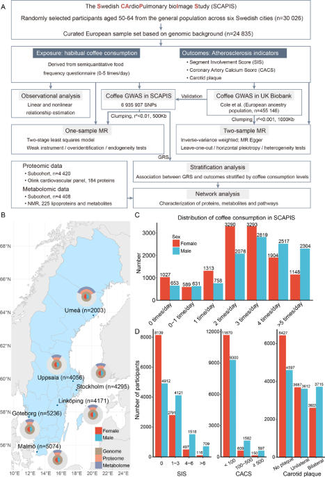
This study utilized data from the Swedish CArdioPulmonary bioImage Study (SCAPIS), a national large-scale observational study that randomly recruited 30,026 individuals aged 50–64 from the population in Sweden (https://www.scapis.org/). Participants were recruited from six major Swedish cities, including Uppsala, Umeå, Linköping, Göteborg, Malmö/Lund and Stockholm between 2013 and 20185,26. The examinations were conducted at the six corresponding university hospitals, and all the examinations were performed on either two or three occasions within a two-week period. No exclusion criteria were applied when recruiting participants, except for the inability to understand spoken and written Swedish for informed consent26.
A comprehensive 140-question survey was designed to gather detailed data on self-reported health, family history, medication, occupational and environmental exposure, lifestyle, psychosocial well-being, socio-economic status, and other social determinants. Additionally, a 35-question food-frequency questionnaire (Mini-Meal-Q) was utilized26.
A 100 mL venous blood sample was collected from participants after an overnight fast for immediate analysis and biobank storage for future analysis26.
All SCAPIS participants provided written informed consent. Ethical approval for this study was obtained from the Swedish Ethical Review Board (2023–01559-01).
To minimize population stratification and ensure the validity and generalizability of the results, we focused on the analysis of participants of European ancestry. The selection was based on a principal component analysis (PCA) that combined the genome data from SCAPIS with the 1000 Genomes (1000G) (https://www.ebi.ac.uk/eva/?eva-study=PRJEB30460) and also accounted for participants’ parental birth countries. In total, 24,835 individuals with European ancestry were included in this study.
Assessment of coffee consumption
A semiquantitative food frequency-questionnaire consisting of 35 questions, known as the Mini-Meal-Q, was employed to gather dietary information, including coffee consumption. Participants were inquired about the frequency at which they typically consume coffee, provided they drank it at least once a month. The available frequency options included never, 1–3 times a month, 1–2, 3–4, 5–6 times a week or 1,2,3,4,5 times a day. These options were converted into continuous numbers and estimated as average daily levels, as follows: 0, 0.067, 0.21, 0.50, 0.79, 1, 2, 3, 4 and 5 times per day, respectively.
SIS measurements
SIS is a semiquantitative measure of the atherosclerosis burden in the coronary arteries, calculated using contrast-enhanced CCTA. In SCAPIS, cardiac imaging was assessed using electrocardiogram gated Computed tomography (CT) imaging at 120 kV. The CT that was obtained was a dual source CT scanner equipped with a stellar detector, (Somatom Definition Flash, Siemens Medical Solution, Forchheim, Germany). In preparation for imaging of SIS, renal function was elevated to identify contraindications and exclude participants at risk of contrast media. The participants also received beta blockers for heart rate deducing purpose, sublingual nitroglycerin for inducing vasodilation and an intravenous injection with contrast in preparation for CCTA5.
SIS has been demonstrated to be a strong and independent predictor of cardiovascular events and has shown superior efficacy in detecting atherosclerosis compared to CACS. The measurement reflects the total extent of coronary segments affected by atherosclerosis, regardless of the stenosis severity, with SIS representing the number of involved segments5,27.
CACS measurements
CACS is a quantitative measure of calcium deposits in the coronary arteries, serving as an indicator of the burden and risk of coronary atherosclerosis. An increasing plaque burden correlates with higher cardiovascular risk, and CACS is valuable for guiding medical treatment and primary prevention strategies in high-risk asymptomatic patients28. Therefore, clinical significance of CACS has incremental prognostic value over conventional risk stratification when predicting future cardiovascular events29 and prediction of all-cause mortality30, making the measurement a strong and independent marker for subclinical heart disease31.
Images for analyzing CACS were obtained by using the same CT scan as for SIS, but without contrast media5. Based on the density and area of the calcium deposits on CT images, the deposits can be quantified using a scoring system, Agaston scoring system32,33,34.
Carotid plaque measurements
Carotid plaque is a useful marker for cardiovascular risk since the measurement reflects not only the atherosclerotic process in the coronary arteries but also the atherosclerotic burden in other parts of the body. The noninvasive measurement of carotid plaque score is considered a strong predictor of major cardiovascular events35 and an independent risk factor for all causes and cardiovascular mortality6.
Atherosclerosis in the carotid arteries were imaged using the two-dimensional greyscale ultrasound (Acuson S2000 ultrasound scanner equipped with a 9L4 linear transducer) and ultrasound images were analyzed shortly after each examination by several operators. The assessment of plaque findings was categorized into three groups: no carotid plaque, unilateral carotid plaque/s and bilateral carotid plaques26. In the analysis, the carotid plaque measurements were converted into numerical values of 0, 1 and 2 respectively.
Genome-wide SNP genotyping
Whole blood samples from different collection sites were randomized before DNA extraction to reduce extraction bias. Two robots (Hamilton Chemagic Star with Chemagen 96-head) performed DNA extraction via magnetic bead separation using Perkin Elmer reagent kit (CMG-1765-A, Lot No. B400-0126110). The quantity of extracted DNA was determined by UV spectrum analysis with Trinean DropSense 96 Polychromatic microplate reader (Techtum).
The DNA samples were genotyped using a customized version of the Illumina GSA-MDv3 at the SNP&SEQ Technology Platform in Uppsala. Genotypes were called with the GenomeStudio software (2.0.3). Finally, the imputed genotype dataset was prepared based on the Haplotype Reference Consortium r1.1 reference panel. The quality control (QC) for genetics data includes (i) genotyping calling rate > 98, (ii) unrelated samples to the 3rd degree, (iii) adjusted heterozygosity falling within three standard deviations of the mean, (iv) no sex test errors and no sex chromosome aneuploidies.
In genomic data preprocessing, SNPs were kept based on an information score greater than 0.7, Hardy–Weinberg equilibrium p greater than 1e-6, and a minor allele frequency threshold of greater than 0.01 was applied to exclude rare variants. Additionally, SNPs and samples with a missing rate of less than 5% were included. In the end, a total of 6.9 million SNPs remained for subsequent analysis.
Targeted proteomics
Proteomic data were generated from EDTA plasma samples with the Olink platform (Olink Proteomics, Uppsala, Sweden). A total of 184 proteins in panel Olink Target 96 Cardiovascular II (v. 5003) and Olink Target 96 Cardiovascular III (v. 6111) were measured using Proximity Extension Assay. The data was presented as normalized protein expression values. The inclusion criteria for proteomic analysis included obtaining completed informed consent and having performed: cardiac computed tomography angiography (CCTA) (or not performed CCTA due to low estimated glomerular filtration rate, estimated glomerular filtration rate (eGFR, < 50 ml/min)), computed tomography (CT) chest, ultrasound carotid arteries, accelerometer data and a complete questionnaire on smoking. The samples were included in a consecutive manner, beginning with the earliest available date for each site.
Nuclear magnetic resonance-based metabolomics
The high-throughput nuclear magnetic resonance (NMR) metabolomics platform Nightingale (Helsinki-Finland, https://nightingalehealth.com)36 was applied to measure the plasma levels of 225 biomarkers including lipoprotein subclasses, lipids and small molecules in EDTA baseline plasma samples. More specifically, the Nightingale panel included (i) absolute quantitative measurements of lipids , lipoproteins, lipid content in lipoprotein particles, and small metabolites, all presented in mmol/L and (ii) the relative measurements of lipid content in each lipoprotein, defined as the lipid fraction relative to the total lipid content within the lipoprotein.
The inclusion criteria for metabolomic profiling were identical to those for proteomic analysis, ensuring a consistent approach to participant selection.
GWAS of coffee consumption
PLINK2 (v 2.00-alpha-2–20190429) was applied to perform GWAS of coffee consumption in SCAPIS. The minimum frequency of SNP was set as 0.01. The covariates included sex, age, site, the first ten principal components of the genome, body mass index (BMI), smoking status, educational level, alcohol consumption habit, physical activity level and marital status. The same set of covariates was applied uniformly across all SNP-level association tests. For the GWAS results of males and females, the analysis was conducted separately for male and female participants, while keeping all other parameters consistent. The Manhattan plots were generated using R package CMplot (v 4.5.1).
The relationship between rs4410790/rs2472297 and coffee consumption was validated by general linear models, with sex, age, BMI, site, smoking status, educational level, alcohol consumption habit, physical activity level and marital status as covariates. The calculation and visualization of coffee consumption partial residuals were performed by R package visreg (v 2.7.0).
The linkage disequilibrium correlation information was extracted from the 1000 Genomes phase 3 reference panel (European population) by ieugwasr package (v 1.0.1).
The GWAS of coffee consumption in UK Biobank was sourced from previously published research results37. In this research, analysis was conducted on a homogeneous European ancestry population (n = 455,146). The covariates included genotyping array and the first 10 genetic principal components.
Mendelian randomization analysis
MR analysis was conducted under three core instrumental variable assumptions: relevance (the instrument is associated with the exposure), independence (the instrument is independent of confounders), and exclusion restriction (the instrument affects the outcome through the exposure). For sensitivity analyses of one-sample MR, an endogeneity test was conducted under the assumption that the exposure is exogenous, and an overidentification test was performed under the assumption that all instruments are valid and consistent with the assumptions of independence and exclusion restriction. And for two-sample MR, sensitivity analyses were conducted under the assumptions that no single instrument unduly influences the estimate (leave-one-out), that instruments affect the outcome only through the exposure (horizontal pleiotropy analysis), and that effect estimates are consistent across instruments (heterogeneity analysis).
Carotid plaque was transformed into a continuous variable with the same method applied in the observational analysis. CACS was divided by 100 before one-sample Mendelian randomization (MR) to place the coefficients on a comparable scale for visualization. One-sample MR was performed by AER package (v 1.2–10, ivreg function), and rs4410790, as well as rs2472297 were instrumental variables (r2 < 0.01 and a 500 Kb window). Sex, age, site and the first ten principal components of genome were included as covariates to maintain the consistency of MR estimation. Two-stage least squares estimation was used as the main statistical model. The weak instrument test, endogeneity test, and overidentification test were provided through the diagnostic summary of the model constructed with the ivreg function. The power calculation for MR estimation was performed with an online tool (https://shiny.cnsgenomics.com/mRnd/)38. The phenotypes associated with the SNPs were retrieved from the GWAS Catalog (https://www.ebi.ac.uk/gwas/home).
For two-sample MR, the significant SNPs associated with coffee consumption in the UK biobank were clumped with a 1000 Kb window and a maximum r2 of 0.001 (the 1000 Genomes phase 3 reference panel [European population]). After clumping, a total of 30 SNPs remained that were shared between the two cohorts. The summarized level GWAS results between the 30 SNPs and three atherosclerosis indicators of SCAPIS were generated by PLINK2 (v 2.00-alpha-2–20190429), and the covariates included sex, age, site and the first ten principal components in the analysis. MRPRESSO (v 1.0) was applied to identify outliers before estimation. Before and after removing outliers, two-sample MR was performed with TwoSampleMR package (v 0.6.4). The inverse-variance weighted (IVW) method and MR-Egger were selected as the estimation model. The three sensitivity analyses, including leave one out sensitivity analysis, horizontal pleiotropy analysis and heterogeneity analysis, were conducted with TwoSampleMR package (v 0.6.4). The single SNP analysis and forest plot visualization were performed with TwoSampleMR package (v 0.6.4).
Genetic risk score construction and stratification analysis
Among the significant SNPs that were associated with coffee consumption in SCAPIS, rs4410790 and rs2472297 were retained after clumping. The genetic risk score (GRS) for coffee consumption was calculated by summing the products of each participant’s effect allele counts at the rs4410790 and rs2472297 loci and the respective coefficients derived from the SCAPIS coffee GWAS. GRS was positively correlated with coffee consumption frequency (the Pearson correlation coefficient of 0.10, p value < 2.2e-16). The relationships between GRS and three atherosclerosis indicators were estimated using general linear models, separately at different coffee consumption levels, and sex, age, BMI, site, smoking status, educational level, alcohol consumption habit, physical activity level and marital status were adjusted in the estimation. The generalized additive model was applied to investigate the relationship between SIS and the interaction of coffee consumption and GRS, using a tensor product smooth with a basis dimension of 3. The same covariates were adjusted for in the generalized additive model. The partial residuals were calculated and visualized with visreg (v 2.7.0).
Multi-omics network analysis
The relationships between GRS and measured proteins/metabolites were estimated using general linear models, with covariates adjusted consistently with those in stratification analysis. Proteins and metabolites with a p value of less than 0.025 were identified as associated with GRS, resulting in the selection of 6 proteins and 54 metabolites, and further network analysis was conducted on these proteins and metabolites.
The pQTL annotations for the 6 proteins were retrieved from https://metabolomics.helmholtz-munich.de/ukbbpgwas/39. The p value threshold was set as 5e-8. Linkage disequilibrium between the reported pQTLs and the variants used to construct the GRS was assessed using the 1000 Genomes phase 3 reference panel (European population) via ieugwasr package (v 1.0.1).
The associations between proteins and metabolites were identified with general linear models, and sex, age, as well as sites were adjusted for. The Benjamini–Hochberg method was employed to conduct multiple hypothesis testing, adjusting the p value to control the false discovery rate (FDR). Associations with FDR of less than 1e-6 were retained. Package igraph (v 2.0.2) was used to construct the network, calculate the degree of each protein/metabolite, and identify the communities (using the fast greedy algorithm and utilizing the absolute values of the regression coefficients as weights). The community structure provided a compact, descriptive summary to organize the protein-metabolite associations and to inform community-level annotation. Package qgraph (v 1.9.8) was applied to implement the Fruchterman-Reingold layout algorithm, and the visualization of network was completed with igraph. The association between proteins/metabolites and SIS was estimated using a general linear regression model, adjusting for the effects of age, sex, and site. Proteins with a p value of less than 0.05 and metabolites with a p value of less than 0.01 were selected for visualization in forest plots. This selection involved two steps: applying the p value criteria and ensuring that the associations with SIS and GRS were directionally consistent. In forest plots, the proteins and metabolites were ranked in descending order based on their degree in the network analysis. The calculation and visualization of SIS partial residuals were conducted with visreg (v 2.7.0).
Statistical analysis
Participants with missing values in any of the measurements or covariates were excluded from the corresponding analysis. General linear models were applied to estimate the effect of coffee consumption on clinical indicators (stats package, R, v 4.3.1). The values of clinical indicators were standardized to z-scores (mean‑centered and scaled by the sample standard deviation) before analyzing. The models were adjusted for sex, age, BMI, site, smoking status, educational level, alcohol consumption habit, physical activity level and marital status. The forest plot was generated using the forestplot package (v 3.1.3) in R.
For the observational association analysis between coffee consumption and three atherosclerosis outcomes, to ensure that the estimated coefficients are on a comparable scale for visualization, CACS was divided by 100 before analysis for linear estimation. For carotid plaque, the absence of plaque was transformed to 0, while unilateral and bilateral carotid plaques were transformed to 1 and 2, respectively. For linear and non-linear estimation, general linear models (stats package, R, v 4.3.1) and generalized additive models (mgcv package, v 1.8–42) were applied. For the multivariable adjusted linear models and non-linear models, sex, age, BMI, site, smoking status, educational level, alcohol consumption habit, physical activity level and marital status were set as covariates. For non-linear models, partial residuals were calculated and visualized by visreg package (v 2.7.0).