
Qubit operation and Bloch sphere representation
A quantum bit, or qubit, is the fundamental unit of information in quantum computing. Unlike a classical bit, which can represent only one of two discrete values (0 or 1), the state of a qubit can exist in an infinite number of possible values. This is because a qubit’s state is a linear combination of the two basis states, denoted by \(|\left. 0 \right\rangle\) and \(|\left. 1 \right\rangle\) as expressed in Eq. (1)25.
$$|\left. q \right\rangle =a|\left. 0 \right\rangle +b|\left. {\text{1}} \right\rangle$$
(1)
Where α and β are the probability amplitudes of the qubit state. The eigenstates \(|\left. 0 \right\rangle\) and \(|\left. 1 \right\rangle\) can also be expressed in two-dimensional vector space in Eqs. (2) and (3)26.
$$a\,=\,R{e_{|\left. 0 \right\rangle }}+iI{m_{|\left. 0 \right\rangle }}$$
(2)
$$b\,=\,R{e_{|\left. {\text{1}} \right\rangle }}+iI{m_{|\left. {\text{1}} \right\rangle }}$$
(3)
Where \(Re_{{|\left. 0 \right\rangle }}\) and \(Im_{{|\left. 0 \right\rangle }}\) are the real and imaginary components of α, \(Re_{{|\left. {\text{1}} \right\rangle }}\) and \(Im_{{|\left. {\text{1}} \right\rangle }}\) are the real and imaginary components of β, and i is an imaginary number, such that i2 = − 1.
Several quantum operators are capable of manipulating a qubit’s state. These quantum operators, often referred to as gates, can be represented using four fundamental Hermitian matrices, known as the Pauli matrices. The Pauli matrices are defined in Eq. (4) through (7) and serve as the building blocks for many quantum operations.
$${\sigma _0}=\left( {\begin{array}{*{20}{c}} 1&0 \\ 0&1 \end{array}} \right)$$
(4)
$${\sigma _x}=\left( {\begin{array}{*{20}{c}} 0&1 \\ 1&0 \end{array}} \right)$$
(5)
$${\sigma _y}=\left( {\begin{array}{*{20}{c}} 0&{ – i} \\ i&0 \end{array}} \right)$$
(6)
$${\sigma _z}=\left( {\begin{array}{*{20}{c}} 1&0 \\ 0&{ – 1} \end{array}} \right)$$
(7)
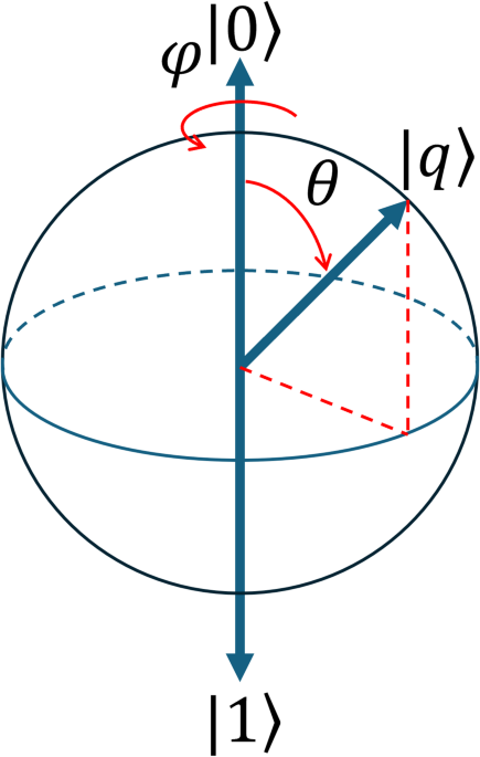
A single qubit state is represented in the 3D space using the Bloch sphere27,28 (Fig. 1). Rotations by angles λ, θ, \(\:\varphi\:\) and around the x, y, and z axis, are performed using the transformation matrix defined in Eqs. (8) through (10), also expressed using the Pauli matrices.
$$RX\left( \lambda \right)=cos\frac{\lambda }{2}{\sigma _0} – isin\frac{\lambda }{2}{\sigma _x}$$
(8)
$$RY\left( \theta \right)=cos\frac{\theta }{2}{\sigma _0} – isin\frac{\theta }{2}{\sigma _y}$$
(9)
$$RZ\left( \varphi \right)=cos\frac{\varphi }{2}{\sigma _0} – isin\frac{\varphi }{2}{\sigma _z}$$
(10)
Fig. 1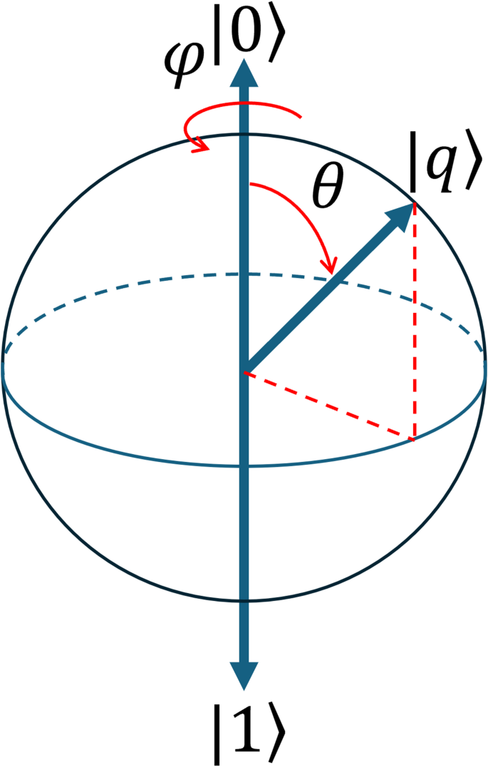
Bloch sphere representation (image adapted from26).
Forward kinematics calculations with quantum circuits
We propose a method for performing forward kinematics calculations using the Bloch sphere representation of qubits. The Bloch sphere allows qubits to represent points in three-dimensional space, and by utilizing this property, we can represent the posture of each link in a robot, which typically consists of multiple links, using qubits. As discussed in previous works15,16, this approach leverages the inherent geometric properties of quantum states to map robotic movements into a quantum framework, enabling new possibilities for efficient calculations in robotic control systems. This enables the representation of the positions of the tips of each link as seen from the root of the robotic structure. By summing the coordinate representations of the qubits corresponding to each link, we can effectively perform a forward kinematics calculation. The corresponding equations for the forward kinematics of a simple manipulator with two links are given in Eqs. (11) and (12).
$$x\,=\,{L_{\text{1}}}{\text{cos}}{\theta_{\text{1}}}\,+\,{L_{\text{2}}}{\text{cos}}({\theta_{\text{1}}}\,+\,{\theta_{\text{2}}})$$
(11)
$$y\,=\,{L_{\text{1}}}{\text{sin}}{\theta_{\text{1}}}\,+\,{L_{\text{2}}}{\text{sin}}({\theta_{\text{1}}}\,+\,{\theta_{\text{2}}})$$
(12)
where L1 is the length of the link 1, L2 is the length of the link 2, θ1 is the joint angle of the joint 1 in the horizontal plane and θ2 is the joint angle of the joint 2 from the link 1 in the horizontal plane.
We designed a quantum circuit to perform forward kinematics calculations by assigning a qubit to each link of a two-link manipulator. Specifically, qubits q0 and q1 represent the posture of link 1 and link 2, respectively. To match the orientation vector of the robot’s links in 3D space with the corresponding vector in the Bloch sphere representation, we applied rotation gates to the qubits. These gates perform rotations in the Roll (X), Pitch (Y), and Yaw (Z) directions within the 3D space, thereby rotating the qubit vectors. In cases where a joint can rotate in multiple directions, the rotation gates in each direction are applied sequentially, as outlined in Eq. (13). Quantum rotations are typically executed as unitary operations on quantum states, with the sandwich product being used when calculating the expectation value or the measured value of the system. This method ensures that the quantum representation of the manipulator’s posture in 3D space remains consistent with the physical behavior of the robot.
$${q_{0 – rotated}}=RX({\lambda_0}) * RY({\theta_0}) * {q_0}$$
(13)
For a serial link manipulator, the absolute position of the tip of a given link is determined by the rotation of all preceding joints. Therefore, the state of the qubit representing the second link must account for the rotation of the first link. Accordingly, the qubit representing the tip position of the second and subsequent links in absolute space, as observed from the root, corresponds to the cumulative effect of all rotation gates involved. This includes the rotation gate of the root link, and the overall transformation is represented by the product of these rotation gates, applied in sequence as detailed in Eq. (14). The sequence of operations, including the quantum rotation gates, reflects the coupled nature of quantum states that represent each link’s posture in the manipulator, which is integral to solving forward kinematics using quantum computing methods.
$${q_{{\text{1}} – rotated}}=RX({\lambda_0}) * RY({\theta_0}) * RY({\theta_{\text{1}}}) * {q_{\text{1}}}$$
(14)
If the posture of a link is represented by a qubit, the expected value of the qubit’s state, when measured with respect to the X, Y, and Z rotation gates, corresponds to coordinates on the Bloch sphere. Given that the radius of the Bloch sphere is unity in this representation, the link distance in absolute space is calculated on a classical computer by multiplying the expected value derived from the qubit by the link length associated with that qubit. As outlined earlier, each link’s posture is encoded by a qubit, and on a conventional computer, the expected values for each qubit are multiplied by their respective link lengths and summed to compute the end-effector position of the manipulator (Fig. 2). In this study, the quantum circuits were implemented using Qiskit, a widely used library for quantum circuit computation29.
Fig. 2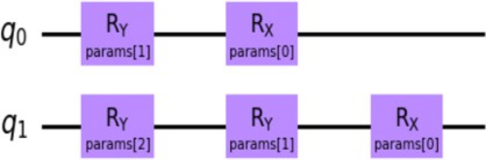
Quantum Circuit for representing 2-link manipulator.
Inverse kinematics calculations with a quantum optimization algorithm (QOA)
For solving inverse kinematics, the conventional inverse matrix method is applicable only when the robot has a small number of degrees of freedom and a unique inverse kinematics solution exists. In contrast, the pseudo-inverse matrix method, which employs optimization techniques, is used to identify the inverse kinematics solution that best satisfies additional constraints in the case of multiple solutions, typically for robots with a higher number of degrees of freedom. This research was inspired by the capability to perform forward kinematics calculations using quantum circuits, and it is hypothesized that faster inverse kinematics calculations for robots could reduce the computational time required for numerous inverse kinematics evaluations during the generation of complex robotic movements.
We propose a method for inverse kinematics computation leveraging forward kinematics quantum circuits and a quantum optimization algorithm. In the field of quantum algorithms, various methods such as Variational Quantum Eigensolver (VQE) and Quantum Approximate Optimization Algorithm (QAOA) have been explored for practical quantum computing applications. These methods typically partition the computational tasks between quantum circuits for solving the quantum mechanical components and classical algorithms for evaluating the results, due to the current limitations of quantum circuits, which are not yet capable of performing long calculations on their own.
In the method proposed in this paper, the inverse kinematics calculation is performed by combining forward kinematics calculations using quantum circuits with convergence determination via classical optimization. First, the quantum circuit is employed to compute the forward kinematics of a robot for a given set of joint angles. Second, the difference between the target end-effector position, calculated classically, and the position obtained from the quantum circuit is evaluated. Third, the joint angles that minimize this difference are computed, and the quantum computation is repeated iteratively until the difference becomes less than a specified threshold. While there are various optimization methods available, this study utilizes COBYLA (Constrained Optimization BY Linear Approximation) as the optimization solver for the quantum optimization algorithm, primarily because it integrates seamlessly with Qiskit. Since the optimization step is carried out classically, additional terms such as energy minimization30 and obstacle avoidance31 can be incorporated into the objective function.
Entangled quantum circuit with RXX, RYY, RZZ gates
For more practical applications, it would be desirable to solve the problem even when the robot has a larger number of degrees of freedom. However, as previously mentioned, inverse kinematics calculations for robotic arms with more than three degrees of freedom cannot be solved geometrically due to the existence of multiple solutions. Therefore, the optimization approach utilizing quantum circuits proposed in this study may offer a promising solution. In the case of a robotic arm with three degrees of freedom per joint and two joints, resulting in a total of six degrees of freedom, a quantum circuit can be constructed as described in Eqs. (15) and (16) (Fig. 3).
$${q_{0 – rotated}}=RX({\lambda_0}) * RY({\theta_0}) * RZ(\varphi ) * {q_0}$$
(15)
$${q_{{\text{1-}}rotated}}=RX({\lambda_0}) * RY({\theta_0}) * RZ(\varphi_{\text{0}}) * RX({\lambda_{\text{1}}}) * RY({\theta_{\text{1}}}) * RZ(\varphi_{\text{1}}) * {q_{\text{1}}}$$
(16)
Fig. 3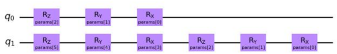
Quantum circuit for representing 2-link 6-DOF manipulator.
However, to fully exploit the potential of quantum computing, entanglement is crucial, as calculations with two independent qubits cannot fully leverage the advantages of quantum computation. In previous approaches, rotation gates that represent the rotation of each link in different directions were applied independently to each qubit. However, in our approach, we utilize the RXX, RYY, and RZZ gates, which apply the same rotation gate to two qubits simultaneously (Fig. 4). For instance, the RXX gate is defined as in Eq. (17).
$$RXX\left( \lambda \right)={\text{exp}}\left( { – i\frac{\lambda }{2}{\sigma _x} \otimes {\sigma _x}} \right)$$
(17)
where \({\sigma _x}\) is the Pauli-X operator, and λ is the rotation angle. The RXX gate acts on two qubits simultaneously, applying the Pauli-X operator to both qubits. This operation introduces a correlation between the two qubits. The Eq. (17) can be transformed to Eq. (18).
$$RXX\left( \lambda \right)=\cos \frac{\lambda }{2}{\sigma _0} \otimes {\sigma _0} – i\sin \frac{\lambda }{2}{\sigma _x} \otimes {\sigma _x}$$
(18)
Entanglement arises between the two qubits due to their inability to behave independently of each other. Specifically, the qubit representing the first link becomes entangled with the qubit representing the second link. This entanglement facilitates a natural representation of a scenario where the rotation of the parent link influences the child link, which in turn reduces the overall computation time. The RX, RY, RZ, RXX, RYY, and RZZ gates, parameterized by angles \(\lambda\), \(\theta\), \(\varphi\), and acting around the x, y, and z axes, are described by equations (19) through (24). While a single-qubit arbitrary rotation gate can be represented as a 2 × 2 unitary matrix, a two-qubit arbitrary rotation gate is generally represented by a 4 × 4 unitary matrix. This enables the manipulation of two qubits in arbitrary ways, allowing for the generation of complex entanglements and interactions.
$$RX\left( \lambda \right)=\left( {\begin{array}{*{20}{c}} {\cos \frac{\lambda }{2}}&{ – i\sin \frac{\lambda }{2}} \\ { – i\sin \frac{\lambda }{2}}&{\cos \frac{\lambda }{2}} \end{array}} \right)$$
(19)
$$RY\left( \theta \right)=\left( {\begin{array}{*{20}{c}} {\cos \frac{\theta }{2}}&{ – \sin \frac{\theta }{2}} \\ {\sin \frac{\theta }{2}}&{\cos \frac{\theta }{2}} \end{array}} \right)$$
(20)
$$RZ\left( \varphi \right)=\left( {\begin{array}{*{20}{c}} {{e^{ – i\frac{\varphi }{2}}}}&0 \\ 0&{{e^{i\frac{\varphi }{2}}}} \end{array}} \right)$$
(21)
$$RXX\left( \lambda \right)=\left( {\begin{array}{*{20}{c}} {\cos \frac{\lambda }{2}}&0&0&{ – i\sin \frac{\lambda }{2}} \\ 0&{\cos \frac{\lambda }{2}}&{ – i\sin \frac{\lambda }{2}}&0 \\ 0&{ – i\sin \frac{\lambda }{2}}&{\cos \frac{\lambda }{2}}&0 \\ { – i\sin \frac{\lambda }{2}}&0&0&{\cos \frac{\lambda }{2}} \end{array}} \right)$$
(22)
$$RYY\left( \theta \right)=\left( {\begin{array}{*{20}{c}} {\cos \frac{\theta }{2}}&0&0&{i\sin \frac{\theta }{2}} \\ 0&{\cos \frac{\theta }{2}}&{ – i\sin \frac{\theta }{2}}&0 \\ 0&{ – i\sin \frac{\theta }{2}}&{\cos \frac{\theta }{2}}&0 \\ {i\sin \frac{\theta }{2}}&0&0&{\cos \frac{\theta }{2}} \end{array}} \right)$$
(23)
$$RZZ\left( \varphi \right)=\left( {\begin{array}{*{20}{c}} {{e^{ – i\frac{\varphi }{2}}}}&0&0&0 \\ 0&{{e^{i\frac{\varphi }{2}}}}&0&0 \\ 0&0&{{e^{ – i\frac{\varphi }{2}}}}&0 \\ 0&0&0&{{e^{i\frac{\varphi }{2}}}} \end{array}} \right)$$
(24)
Fig. 4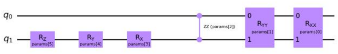
Quantum Circuit for representing 2-link 6-DOF manipulator with RXX, RYY, and RZZ gates.
Mathematically, if the state of a two-qubit system cannot be represented as a single tensor product of the individual qubit states, it is considered to be in an entangled state. As shown in Eq. (18), the RXX gate transforms the system into a state that is a superposition of tensor products, which is an entangled state. The degree of entanglement, quantified by the concurrence32, varies depending on the angle λ33. Notably, when λ equals π/2, the system is in a Bell state, which represents the maximum entangled state. In Qiskit, the implementation of a two-qubit rotational gate is achieved through a decomposition into a series of Hadamard, CNOT, and RZ gates. This decomposition is advantageous because it allows for efficient execution on quantum hardware that natively supports these fundamental gates. The corresponding unitary transformation can be realized through the following gate sequence:
1.
Apply Hadamard gates to both qubits.
2.
Apply a CNOT gate with the first qubit as the control and the second as the target.
3.
Apply an RZ gate to the target qubit.
4.
Apply another CNOT gate.
5.
Apply Hadamard gates to both qubits again.