
Data processing and evaluation as well as statistical analyses were performed in software R 4.2.1 [16]. Genotype preparation, phasing, imputation and population analysis were done by using PLINK 1.9 and PLINK 2.0 [17] and Beagle 5.4 [18, 19]. ASReml-R 4.1.0 [20] was used for univariate estimation of breeding values and GCTA 1.94.1 [21] for GWAS with de-regressed GEBVs as phenotypes.
Materials
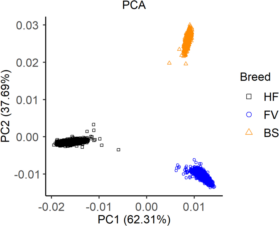
The dataset consists of 5,703 dairy cows of the breeds German Holstein (HF, \(n=\) 2,300), German Fleckvieh (FV, \(n=\) 2,330) and German Brown Swiss (BS, \(n=\) 1,073), originating from 48 farms. The farms are members of the breeding organization Rinderunion Baden-Württemberg e.V. (Herbertingen, Germany) and work with automatic milking systems. The milking data, consisting of yield per milking and start time of milking, from the automatic milking systems were longitudinally recorded between October 2017 and April 2024 and were provided by the Landeskontrollverband Baden-Württemberg e.V. (Stuttgart, Germany).
Animals in our study were genotyped with 50 K SNP chips. For HF, the Eurogenomics-MD-Chip was used in several versions. The merging of the chips and the imputation of undetermined SNPs were done by Vereinigte Informationssysteme Tierhaltung w.V. (Verden, Germany). Genotyping of FV and BS was done by Landeskontrollverband Bayern (Munich, Germany) and Bayerische Landesanstalt für Landwirtschaft (Grub, Germany) using Illumina BovineSNP50v2 BeadChip or DAC-BS50 Illumina. For both breeds, we obtained a standardized data set over the different chips, whereby missing SNPs were called with the population mean. We excluded SNPs on sex chromosomes, on undefined position, with minor allele frequency (MAF) < 0.03 or missing call rate > 0.01. The MAF threshold was stricter than in comparable studies [13, 22] in order to cause fewer false-positive results in the GWAS and was based on a study with a similar data set to our BS sample [23]. SNPs that are not included in the high-density reference panels were excluded, as they would be automatically removed during imputation. All genotypes were updated to the reference genome assembly ARS-UCD1.2 by manually replacing the existing coordinates with the updated ones [24]. SNPs, which are not listed in the ARS-UCD1.2, were excluded. This left 31,416 SNPs for HF, 34,238 SNPs for FV and 31,527 SNPs for BS.
A detailed overview of the size of the raw genotype and phenotype data and remaining data sets after filtering per breed can be found in the Supplementary (see Additional File 1).
MethodsCalculation of resilience indicator traits
Milk yields per milking were added up to daily milk yields, whereby the first milking was divided proportionally between the current and the previous day. Daily milk yields were filtered as follows. Days where the number of animals milked on the farm deviated by three standard deviations from the mean number of animals normally milked on the farm as well as the day before and after were removed for all animals on this farm. Furthermore, the day before and after an individual gap of an animal, meaning one or more days without available data, was removed. Lactations were considered from day 10 to day 305, and those with less than 50% coverage respectively 148 data points were excluded. For each lactation of each cow, a lactation curve was predicted using spline interpolation with pspline in R [25] with degrees of freedom set to 5 and data points weighted by the strength of assumed disturbances. Details are described in Keßler et al. [6].
We considered three resilience indicator traits. The variance of the deviations between observed and predicted absolute daily milk yield (\({v}_{d}\)) was calculated as:
$${v}_{d}\left({\mathbf{y}}_{il}\right)=\frac{1}{n-1}*\sum_{t=10}^{n}{\left(\left({{\varvec{y}}}_{{\varvec{i}}{\varvec{l}}{\varvec{t}}}-{\widehat{{\varvec{y}}}}_{{\varvec{i}}{\varvec{l}}{\varvec{t}}}\right)-\overline{\left({{\varvec{y}}}_{{\varvec{i}}{\varvec{l}}}-{\widehat{{\varvec{y}}}}_{{\varvec{i}}{\varvec{l}}}\right)}\right)}^{2}$$
with \({\varvec{y}}\) a \(n\)-vector with daily milk yields of a cow \(i\) in a certain lactation \(l\), \(\widehat{\mathbf{y}}\) the vector with interpolated daily milk yields and \(t\) the lactation day. The variance of relative daily milk yields (\({v}_{r}\)) in considered lactation period was calculated as:
$${v}_{r}\left({\mathbf{y}}_{il}\right)=\frac{1}{n-1}*\sum_{t=10}^{n}{\left(\left({\alpha }_{ilt} {\mathbf{y}}_{ilt}\right)-\overline{\left({\alpha }_{il} {\mathbf{y}}_{il}\right)}\right)}^{2}$$
with \({\varvec{y}}\) a \(n\)-vector with daily milk yields of a cow \(i\) in a certain lactation \(l\) and the scaling factor \({\alpha }_{il}=\frac{100}{\sum_{t=10}^{n}{y}_{ilt}}\) with \(t\) the lactation day. The two parameters were logarithmized to conform to the assumption of normal distribution according to previous analyses in Keßler et al. [6].
The autocorrelation of the deviations between observed and predicted absolute daily milk yield (\({r}_{Auto}\)) was calculated as:
$${r}_{Auto}\left({\mathbf{y}}_{il}\right)=\frac{cov\left({\mathbf{y}}_{il}-{\widehat{\mathbf{y}}}_{il}\right)}{var\left({\mathbf{y}}_{il}-{\widehat{\mathbf{y}}}_{il}\right)}$$
and in detail:
$${r}_{Auto}\left({\mathbf{y}}_{il}\right)=\frac{\frac{1}{n-2}*\sum_{t=2}^{n}\left(\left(\left({{\varvec{y}}}_{{\varvec{i}}{\varvec{l}}{\varvec{t}}}-{\widehat{{\varvec{y}}}}_{{\varvec{i}}{\varvec{l}}{\varvec{t}}}\right)-\stackrel{-}{\left({{\varvec{y}}}_{{\varvec{i}}{\varvec{l}}}-{\widehat{{\varvec{y}}}}_{{\varvec{i}}{\varvec{l}}}\right)}\right)*\left(\left({{\varvec{y}}}_{{\varvec{i}}{\varvec{l}},{\varvec{t}}-1}-{\widehat{{\varvec{y}}}}_{{\varvec{i}}{\varvec{l}}{\varvec{t}}}\right)-\stackrel{-}{\left({{\varvec{y}}}_{{\varvec{i}}{\varvec{l}}}-{\widehat{{\varvec{y}}}}_{{\varvec{i}}{\varvec{l}}}\right)}\right)\right)}{\frac{1}{n-1}*\sum_{t=1}^{n}{\left(\left({{\varvec{y}}}_{{\varvec{i}}{\varvec{l}}{\varvec{t}}}-{\widehat{{\varvec{y}}}}_{{\varvec{i}}{\varvec{l}}{\varvec{t}}}\right)-\stackrel{-}{\left({{\varvec{y}}}_{{\varvec{i}}{\varvec{l}}}-{\widehat{{\varvec{y}}}}_{{\varvec{i}}{\varvec{l}}}\right)}\right)}^{2}}$$
Genetic analysis
The resilience indicators described above were genetically analyzed separately for each breed and two different lactation groups. The first one, labelled \(P\) for primiparous, included phenotypes from the first lactation. For the second one, named \(M\) for multiple lactations, we added information also from higher lactations of the cows in \(P\) as repeated measurements. Thus, a univariate analysis was performed for each of six groups: first lactation HF, all lactation HF, first lactation FV, all lactation FV, first lactation BS, all lactation BS. The animal model for the data sets with information about cows in the first lactation was:
with \(y\) vector of observations, \(u\) vector of additive genetic effects, \(e\) vector of residuals, and incidence matrices \(X\) and \(Z\). The animal model for all lactations of the considered cows was:
where \(pe\) is the vector of permanent environmental effects and \(W\) is the incidence matrix. The additive genetic effects \(u\), the permanent environmental effects \(pe\) and the residual effects \(e\) were normally distributed with \(u \sim N(0,G{\sigma }_{u}^{2})\), \(pe \sim N\left(0,{I}_{pe}{\sigma }_{pe}^{2}\right)\) and \(e \sim N\left(0,{I}_{e}{\sigma }_{e}^{2}\right)\), whereby \(I\) are identity matrices. The genomic relationship matrix \(G\) was built according to VanRaden et al. [26]. The vector of fixed effects \(b\) comprises in each model age at first calving in month, herd-year-season effect and completeness of lactation data. In the second model the effect of the lactation separated in first and higher lactation was added. Season in herd-year-season was divided into spring from March to May, summer from June to August, autumn from September to November, and winter from December to February and completeness of lactation data was graded in ≥ 90%, 80%—< 90%, 70%—< 80%, 60%—< 70%, 50%—< 60%. In all analyses, effect levels with fewer than six animals are excluded. This left 1,370 HF cows for \(P\) and 1,538 HF cows for \(M\), for FV 1,135 cows in \(P\) and 1,551 in \(M\) and for BS \(P\) includes data from 310 and \(M\) from 488 cows. For further analysis, we de-regressed the cow’s additive genetic effects, i.e. their GEBV, by dividing the effects by their reliabilities and standardized them to a mean of 0 and a standard deviation of 1 within each group. We also calculated the heritability as the proportion of additive genetic variance of the total variance.
Additionally, a selection index (\(SI\)) was computed that combines the resilience indicators into a single trait. The selection index is a linear combination of the GEBVs of individual resilience indicators, with weights chosen to optimally describe overall resilience. Weighting factors were determined in Keßler et al. [8], by maximizing the selection response in health traits when selecting on resilience indicators based on the performance trait daily milk yield. The weighting factors were adopted from this study, which were estimated in the same data set [8]. The selection index was calculated as
$$SI\left({\mathbf{y}}_{i}\right)=0.65*{\widetilde{v}}_{d}\left({\mathbf{y}}_{i}\right)+ 0.35* {\widetilde{v}}_{r}\left({\mathbf{y}}_{i}\right),$$
where \({\widetilde{v}}_{d}\left({\mathbf{y}}_{i}\right)\) and \({\widetilde{v}}_{r}\left({\mathbf{y}}_{i}\right)\) were GEBVs of the logarithmized, negated \({v}_{d}\left({\mathbf{y}}_{i}\right)\) and \({v}_{r}\left({\mathbf{y}}_{i}\right)\), for cow \(i\). The selection index was calculated in both lactation groups, \(P\) and \(M\), and all three breeds.
Imputation
For further analyses we imputed the 50 K genotypes to high-density genotypes. The following reference panels were used. For HF, we used data from 1,278 Australian Holsteins with 585,517 SNPs that were genotyped with the BovineHD Genotyping BeadChip [27]. High-density data from 3,439 FV cows and bulls including 629,028 SNPs genotyped with Illumina BovineHD Bead chip [28] and 192 BS individuals with 613,140 SNPs genotyped with Illumina Bovine-HD [23] were available. Similar to the 50 K genotype data, SNPs whose MAF was < 0.03, whose missing call rate was > 0.01 or which were found on sex chromosomes were removed. The positions of considered SNPs were updated to the reference genome ARS-UCD1.2 [24]. 522,726 SNPs in HF, 580,873 SNPs in FV and 503,971 SNPs in BS remained.
Reference panel data were phased using beagle 5.4 within each dataset. 50 K and high-density data of each breed were concorded with conform-gt and then imputed with beagle 5.4. According to [29], the effective population size Ne was set to 100. Apart from that, the default settings were used. SNPs with a dosage R-Squared < 0.75 are removed to maintain a sufficiently high imputation quality [19]. The final imputed data set contains 2,300 HF cows with 503,263 SNPs, 2,330 FV cows with 569,056 SNPs and 1,073 BS cows with 493,637 SNPs. For the across-breed population analysis, the imputed genotypes were merged with PLINK 1.9 [30], leaving 401,491 SNPs shared across all breeds.
Population analysis
Population analyses were done in PLINK 1.9 for MDS and PLINK 2.0 for LD analysis [17]. Genomic relationship between the breeds was studied with a MDS based on imputed genotypes, considering only SNPs that remained in all three breeds after all filtering steps described above. The LD was analysed across breeds and breed-specific, using the maximum number of available SNPs in the imputed genotype datasets of each breed, respectively the merged imputed dataset after all filtering steps. The LD was calculated as the \({r}^{2}\) [31]:
$${r}^{2}= \frac{{\left({p}_{{A}_{1}{B}_{1}}-{p}_{{A}_{1}}{p}_{{B}_{1}}\right)}^{2}}{{p}_{{A}_{1}}{p}_{{A}_{2}}{p}_{{B}_{1}}{p}_{{B}_{2}}}$$
with \(p\) the allele frequency, \({A}_{1}\) and \({A}_{2}\) alleles on gene locus \(A\) and \({B}_{1}\) and \({B}_{2}\) alleles on gene locus \(B\). The LD between pairs of SNPs that were a maximum of 1,000 SNPs or 3,000 kilobases apart was calculated.
Genome-wide association study
For each of the six groups defined above, a GWAS was performed for the resilience indicator traits and the selection index. We optimized the GWAS model by minimizing the difference of the genomic inflation factor lambda \({\lambda }_{GC}\) to 1 in each breed. \({\lambda }_{GC}\) is calculated as the ratio between the median of the observed chi-squared test statistics and the expected median of 0.455 [32]. The value should be close to 1 or slightly above [22, 33]. We therefore decided for a mixed linear model based association analysis (\(MLMA\)) for HF, a \(MLMA\) excluding the GRM of the chromosome where the SNP is located (\(MLM-LOCO\)) for BS and a \(MLM-LOCO\) corrected for a fixed effect of the principal components calculated based on the whole genome (\({\text{MLM}-\text{LOCO}}_{PC Genome}\)) to account for population stratification for FV [21] (\({\lambda }_{GC}\) of the selected GWAS are provided in the results, all \({\lambda }_{GC}\) are provided in Additional File 2).
GWAS were performed using the following model:
$$y = \mu + Xb+ Zu + e,$$
with \(y\) vector of de-regressed, standardized additive genetic effects of each animal derived from univariate analysis for each resilience indicator trait and the selection index, the population mean \(\upmu\), fixed effects \(b\) with the incidence matrix \(X\), including the reference allele coded with 0, 1 or 2, the vector of additive genetic effects \(u\) with \(u \sim N(0,G{\sigma }_{u}^{2})\) and \(G\) the genomic relationship matrix created according to Yang et al. [34], and the residual term \(e\) with \(e \sim N(0,{{I}_{e}\sigma }_{e}^{2})\). In \(MLM-LOCO\) and \({\text{MLM}-\text{LOCO}}_{PC Genome}\), \(G\) is calculated for each chromosome separately and leaves out the chromosome, where the SNP to be tested for association is located. The vector \(b\) includes the additive effect of the candidate SNP to be tested for association and for \({\text{MLM}-\text{LOCO}}_{PC Genome}\) in FV a covariate of 20 principal components, which were calculated based on the whole genome with software GCTA [35]. For the calculation of GWAS in GCTA, the reference allele was specified in accordance with ARS-UCD1.2.
For across-breed evaluation, we pooled the p-values in data set \(P\) and data set \(M\) per resilience indicator using the package poolr in R [36]. We used the Fisher method, which is based on the chi2-statistic:
$${X}^{2}=-2\sum_{i=1}^{k}\text{ln}({p}_{i})$$
with K number of tests (three) and pi the p-values of the GWAS.
The results of the single GWAS and pooled GWAS are shown as Manhattan plots, whereby two significance thresholds were defined. Genome-wide significance was determined using Bonferroni correction with, with \(N\) number of SNPs, and a less stringent, suggestive level of significance was set to \(p\le \frac{0.05}{N}\). For SNPs showing significant association at the stringent significance level, the Cattle QTL Database release 53 [27] was used to search for QTL in the range from 25 kB up- and downstream.