Bacteria regulate collective behaviour by mechanosensing cell–cell collisions

Bacterial strains

All strains and plasmids used in this study are listed in Supplementary Table 1. Gene deletions were constructed by two-step allelic exchange54 following published protocols15. Plasmids were constructed using standard Gibson assembly55 and introduced into P. aeruginosa cells by electroporation. Bacteria were then grown in SOC medium (Corning) for 1 h at 37 °C at 210 r.p.m., streaked on Luria–Bertani (LB, Carl Roth) 1.5% agar plates supplemented with gentamycin (60 µg ml−1) and incubated overnight at 37 °C. The next morning, single colonies were checked for fluorescence under the microscope and frozen in 1% dimethyl sulfoxide at −80 °C. Throughout the paper, we refer to the double-mutant ∆pilG cpdA as ∆pilG for simplicity. The cpdA deletion was introduced to restore cAMP levels to WT values, compensating for the reduced piliation and shorter aspect ratio caused by simple pilG deletion15.

Growth conditions

Bacteria from frozen stocks were streaked onto pre-warmed LB agar plates supplemented with gentamycin at 60 µg ml−1 whenever necessary and incubated overnight at 37 °C. A single colony was inoculated into 1 ml filtered LB supplemented with antibiotics if necessary, and cultured overnight at 37 °C at 210 r.p.m. Overnight cultures were diluted to optical density (OD600) 0.05 in 2 ml filtered LB and incubated for 3 h under the same conditions to reach OD600 0.6–0.8 (for example, exponential phase).

For twitching assays, semi-solid tryptone agar plates were prepared by autoclaving 0.55% (w/v) agarose standard (Carl Roth), 10 g l−1 tryptone (Carl Roth) and 5 g l−1 NaCl (Fisher Bioreagents). After cooling the broth to 55 °C for 30 min, 30 ml of the broth was then poured into 90 mm Petri dishes, dried for 30 min at room temperature under the flow hood and stored at 4 °C for 1 day. For twitching assays in micromaze, the same procedure was followed with the tryptone concentration reduced to 1 g l−1.

Single-cell twitching assay

Agarose plates were pre-warmed for 1 h at room temperature and round pads were cut out. Exponential-phase bacterial cultures were diluted to OD600 0.5, and for some experiments, mixed according to the following ratios: 90:10 (non-fluorescent:fluorescent strains) for twitching motility in diluted populations (Extended Data Fig. 5a), 98:2 for twitching motility in dense populations (Fig. 3a), 50:50 (WT:mutant) for competition assays (Fig. 3j, and Extended Data Figs. 6d–h, 7 and 8) unless otherwise stated (Extended Data Fig. 6j,k), and 80:20 (non-fluorescent:fluorescent strains) for leading-edge experiments (Fig. 3h). Of the resulting culture, 2 µl was pipetted onto the surface of the pad. Right after the droplet dried, the pad was flipped onto a glass-bottom dish (MatTek), and PBS droplets were added to the edges to prevent drying. Pads were incubated at 37 °C for 1.5 h, 2.2 h, 3 h or 4.5 h to obtain bacterial populations at low (~10%), medium (~30%) and high (~70%) surface coverage, or to image the leading edge, respectively (see ‘Features quantification’ section). Bacterial motility was monitored under these conditions, as described in the ‘Microscopy’ section.

Design of micromaze

Designs were generated using Klayout software and comprised 21 motifs arranged in three rows within a 40 × 22 mm area, corresponding to a standard coverslip size. Each motif featured a central inlet (diameter ~4 mm) connected radially to ~50 maze-like structures arranged in a circular pattern. Designs were exported as GDS files.

Fabrication of micromaze

Micromaze fabrication was performed at the UC San Diego Nanofabrication Facility using standard photolithography and reactive ion etching of fused silica. Four-inch fused silica wafers (thickness 500 µm, Wafer Pro) were cleaned using RCA procedures (SC1 and SC3), spin rinsed and dried (MEI SRD). AZ 1512 photoresist (EMD Performance Materials) was spin-coated to a thickness of ~0.6 µm and patterned on a Heidelberg MLA system (375 nm, exposure dose 140 mJ cm−2) using the custom GDS design files. The developed wafers (AZ 400, 45 s) were coated with a 200 nm chromium layer deposited at 1 Å s−1 by electron-beam evaporation (Temescal system) and lifted off in RR41, acetone and IPA. The substrates were etched to a depth of 1.2 µm using a PlasmaTherm ICP-RIE system under optimized C4F8/Ar plasma conditions56 (low-pressure, high-power regime; etch rate ≈ 0.26 µm min−1). Feature heights were verified by scanning electron microscopy (Extended Data Fig. 9d). The wafers were diced into 40 × 22 mm pieces for subsequent experiments.

Twitching assay in micromaze

Round pads were cut out from pre-warmed agarose plates using a stamp with a diameter of 12 mm. Overnight bacterial cultures were diluted to OD600 0.2 and dropped to the centre of each pad using a toothpick. Once the droplets had dried, plates were incubated at 37 °C for 5 h. Meanwhile, the glass chip was sequentially cleaned with boiling water, isopropanol and water, then mounted in a custom metal holder compatible with the microscope stage. Before adding bacteria, each design was inspected under the microscope to select one free of agarose residues that could clog the maze features (see Microscopy section). A pad containing a colony with an apparent twitching zone was then flipped onto the selected structure. For the competition experiment (Fig. 4g), WT and ∆pilH were mixed in equal proportion at OD600 0.8. The mixture was dropped to the pad and, once dried, directly flipped onto the selected structure, ensuring an equal proportion of the two strains at the entrance of the maze. Using a custom template, the pad was aligned so that the colony was centred over the motif’s inlet. Alignment was verified under the microscope, ensuring that bacteria were located within the inner circle at the maze entrance, with no cells inside the maze or at the outlet at the start of the experiment. Bacterial motility was then monitored as described in the Microscopy section.

MicroscopyWidefield microscopy

Most experiments investigating twitching motility in open spaces were performed on a widefield microscope (Ti Eclipse, Nikon) equipped with a phase-contrast ring and a ×100 oil-immersion objective (Plan Apo λ, NA = 1.45). A ×20 objective (Plan Apo λ, NA = 0.75) was used for competition assays (Fig. 3j and Extended Data Fig. 6d,g). Images were recorded using a CMOS camera (ORCA-Flash 4, Hamamatsu), with focus maintained by the Perfect Focus System (PFS, Nikon). Image acquisitions were computer controlled using NIS software (v.5.02.03). Twitching motility was monitored using phase contrast, often combined with fluorescence. For fluorescence acquisitions, the LED power was set to 20% and the exposure time to 100 ms. Bacterial motility was monitored at 5-s intervals during 5 min at room temperature.

Spinning-disk microscopy

A spinning-disk confocal microscope (Eclipse Ti2, Nikon) equipped with a spinning-disk module (CSU-W1, Yokogawa) was used for selected experiments, including imaging of the mNeonGreen-PilG fusion protein sensitive to photobleaching (Fig. 3h and Extended Data Fig. 6a,c) and twitching motility in structured environments (Fig. 4b). Images were recorded using a CMOS camera (ORCA-Fusion-BT, Hamamatsu). Acquisition parameters (laser power, exposure time, focus stabilization, software) were identical to those described above. For mechanosensing acquisitions, bacterial motility was imaged using a ×100 oil-immersion objective (Plan Apo λ, NA = 1.45) using both phase contrast and fluorescence modes at 5-s intervals for 5 min. For micromaze experiments, mazes were first mapped in brightfield using a ×20 objective (Plan Apo λD, NA = 0.8) by generating 8 × 8 tiled images of entire designs. Bacterial motility was then recorded in a clean design using a ×40 long-working-distance water-immersion objective (Apo LWD λS, NA = 1.15) in fluorescence at 5-s intervals during 4 h at room temperature. To reduce the amount of data generated, a single brightfield image of the maze structure was acquired at the start of each experiment.

Image analysisQuantification of competition experiments

Images of competing fluorescent strains at the colony front were acquired at ×20 magnification and rotated to align the leading edge perpendicular to the x axis, with the uncolonized area on the right. Background pixels were set to zero, and the edge was defined as the first non-zero pixel along the horizontal direction (set as distance = 0 µm, Fig. 3j and Extended Data Fig. 6d,g). As individual cells could not be resolved, bacterial distribution was inferred from fluorescence profiles. Fluorescence was quantified along lines perpendicular to the edge by counting positive pixels and converted into bacterial numbers using an estimated cell width of ~3 pixels. Values were averaged every 10 pixels, approximating cell length, to estimate bacterial number as a function of distance from the edge. Relative strain abundance was calculated as the fraction of bacterial numbers in each channel relative to the total.

All other quantifications were performed on higher-resolution images acquired at ×40 or ×100 magnification, allowing analysis at the single-cell level. The analysis workflow consisted of three steps: segmentation, single-cell tracking (optional) and quantification of relevant features as described below.

Single-cell segmentation

Single-cell segmentation was performed using Omnipose57 (v.1.0.6) via its Python interface with the model ‘bact_phase_omni’ and parameters ‘mask_threshold=1.75 and flow_threshold=0.4’. For analyses at the leading edge, segmented images were further divided into ‘Edge’ and ‘Core’ regions. The edge, defined as the outer layer where bacteria form ordered rafts, was delineated by measuring the typical raft size in each field of view (~2 5µm) and drawing a manual line of corresponding thickness along the colony boundary. This line was then used to split the segmented images into two movies, one for edge bacteria and one for core bacteria.

Single-cell tracking

Single-cell tracking was used to follow segmented bacteria over time and quantify their dynamic behaviour. Segmented cells were tracked with TrackMate (v.7)58 using the Trackastra algorithm59 previously trained on our data. To minimize tracking errors and manual corrections, only a defined subset of fluorescently labelled cells mixed at a specified ratio (see ‘Single-cell twitching assay’ section) was tracked.

Features quantification

Segmented images were used as inputs to extract quantitative features using custom Python scripts (v.3.9.0), with tracking applied only when stated.

Surface coverage

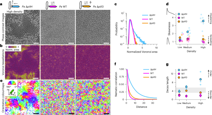
Surface coverage (that is, spatial occupancy or packing fraction) was used as the primary density metric in place of cell density (that is, cell number per unit area) to account for differences in cell size across strains and enable comparison of collective organization under similar physical contact conditions. Surface coverage was quantified as the fraction of pixels occupied by bacteria in microscopy images. Mean surface coverages and corresponding cell densities for each experimental condition shown in Fig. 1g are reported in Supplementary Table 2. Results presented in Fig. 1d,g were also validated at matched cell numbers per unit area (Extended Data Fig. 2). Mean cell numbers per unit area and corresponding surface coverage for each experimental condition shown in Extended Data Fig. 2 are reported in Supplementary Table 3.

Bacterial length and width

For each bacterium, cell length was defined as the Euclidean distance between its two most distant extremities. Cell width was measured along a vector perpendicular to the length axis: all points along this perpendicular line that fell within the cell were identified, and the distance between the two points farthest apart was taken as the cell width.

Bacterial orientation

Bacterial orientation was defined as the angle between the vector connecting the two length extremities and the positive x axis, corrected for the downward-pointing y axis and expressed in degrees from 0 to 360°.

Nematic correlation function

For each cell, the nematic correlation function was determined by identifying neighbours at a radial distance r, computing cos[2(θi − θj)] for all neighbours (θi and θj being the orientations of the cell and the neighbour, respectively) and averaging over all neighbours. These averaged values were then further averaged over all cells to yield the correlation as a function of r. Distances were normalized to the bacterial width.

Decay length

The decay length was determined by fitting the nematic correlation function to an exponential model of the form: a × exp(−r/b) + c, where a represents the amplitude of the correlation function, b is the decay length and c is the asymptotic value at long distances. The decay length reflects the characteristic distance over which the nematic correlation decreases. Fitting was performed using data for r > 2 to ensure the presence of neighbours.

Voronoi tessellation

Bacterial spreading was visualized and quantified using Voronoi tessellation, which partitions spaces, here the segmented image, into tiles containing a single bacterium and all points closer to it than to any other21. Representative points (for example, centroids and contour points) of all the cells were used to generate Voronoi polygons using the Python Voronoi function, assigning each pixel to its nearest cell. Tiles were overlaid on raw images with a colour code indicating tile area, displayed using a plasma colourmap. Tiles at the image edges were excluded from analysis. Polygon areas of remaining cells were computed (denoted as raw Voronoi tile area) and normalized to the mean area of all Voronoi tiles in the image (denoted as normalized Voronoi tile area), providing a measure robust to small differences in bacterial length between strains. The distribution of normalized tile areas was plotted on a logarithmic scale and characterized using its skewness, which quantifies spreading. Uniform spreading was characterized by narrow, symmetric distributions (skewness ≈ 1), whereas spatial heterogeneity was characterized by broader, right-skewed distributions (skewness > 1).

Polarization angle

The mNeonGreen-PilG fusion protein was used to directly assess PilG mechanosensing activity at the leading edge, visible as two fluorescent foci at the poles of the cell15. Images were rotated such that the leading edge was oriented vertically. For each bacterium expressing the mNeonGreen-PilG fusion protein, bacterial polarization, defined as the vector from the centroid to the brighter pole, was determined from fluorescence intensity profiles along the long axis. The polarization angle was measured relative to the x axis pointing towards the uncolonized space, and angles across all cells were summarized in polar histograms.

Heat maps of bacterial residence in mazes

Fluorescence images, acquired with ×40 objective, of bacteria moving in micromazes were rotated and cropped using the brightfield maze image as a reference, so that the final image spanned the full maze width and extended from the top V-shaped inlet to the bottom inverted V-shaped exit. Then, single bacteria were segmented using Omnipose57 (model ‘bact_fluor_omni’, see ‘Single-cell segmentation’ subsection), and segmented images were binarized by setting all pixels >1 to 1. In Fiji (v.2.16), three independent movies of each strain (WT or ∆pilH) were combined to generate a single binary movie per strain. Time projections were obtained by summing all the frames, generating images where pixel values represented the number of frames bacteria occupied for each position. These images were normalized to the total sum of pixel values to generate density heat maps. Density maps were further normalized to the maximum pixel value in the ∆pilH image, resulting in residence probability heatmaps with values from 0 to 1 for ∆pilH and 0 to 0.452 for WT. Final images were displayed using the magenta-hot inverted look-up table.

Surface coverage and escape probability in mazes

To measure surface coverage, the brightfield image of the maze was first used to define the maze contour via Otsu thresholding, edge detection and selection. Then, time projections of the segmented bacteria were thresholded to identify all pixels occupied by bacteria over the course of the 4-h experiment. The maze contour was then applied to calculate the fraction of the maze area covered by bacteria, and values were averaged across replicates for each strain. To measure the escape probability, the segmented image of the maze was used to automatically detect the central maze region (from the entrance to the exit) and the outlet region (from the exit to the bottom of the image). Bacteria within the maze and at the outlet were counted, with the total defined as the sum of these two populations. Escape probability was calculated as 100 × (bacteria at outlet/total bacteria) and averaged across the three replicates for each strain.

Contact reversals

Quantification of the frequency and probability of contact reversals required previous single-cell tracking and extraction of the spots CSV table from TrackMate58 (see ‘Single-cell tracking’ subsection). First, tracks were classified as ‘moving’ if the displacement between consecutive frames exceeded 5 pixels, and only tracks containing at least 3 consecutive moving frames were considered valid. Second, for a given reference bacterium, neighbours were defined as any bacteria in physical contact with it. Contact was determined by drawing a circle of radius 3 px (~0.2 µm) at the leading pole of the reference bacterium. Any bacterium whose label fell within this circle was counted as a neighbour, with each contact event recorded only once. In most cases, a reference bacterium had only one neighbour at a time, although multiple simultaneous contacts were possible. Third, reversals were detected by analysing the trajectory over 5 consecutive frames: the angles between consecutive displacement vectors were computed, and a reversal was recorded when the bacterium moved steadily in one direction for at least 2 frames (angles <90°), then abruptly changed direction (angles >110°), and continued steadily in the new direction for at least 2 frames (angles <90°). Contact reversals were defined as reversals occurring while the bacterium was in contact with one or more neighbours immediately before reversing its motion and were manually checked before further analysis. Three parameters were then computed: the frequency of reversals (that is, total number of reversals divided by total tracked time in hours), the frequency of contact reversals (that is, total number of contact reversals divided by tracked time), and the probability of contact reversals (that is, total number of contact reversals divided by total number of contacts). Total tracked time was defined as the sum of the durations of all trajectories in a movie.

Mean squared displacement

Quantification of MSD used spots CSV tables extracted from TrackMate58 as input (see Single-cell tracking subsection). For each trajectory, MSD was computed from the squared differences in positions separated by a lag time ∆t using the following formula: MSD(∆t) = 〈[x(t + ∆t)−x(t)]2 + [y(t + ∆t)−y(t)]2〉, where the brackets indicate averaging over all valid point pairs separated by ∆t. MSD and time were normalized to unitless values: MSD[unitless] = MSD/characteristic_length2 and t[unitless] = t/characteristic_time, with characteristic_length = 0.8 μm (bacterial width) and characteristic_time = 4 s (time to travel the characteristic length). Ensemble-averaged, normalized MSD curves were obtained by averaging individual MSD curves over time and plotted on a log–log scale. Their scaling behaviour was quantified by fitting a power law, log10(MSD) = a × log10(Δt) + b, where the slope a characterizes motion type. For example, MSD scaling with ta with a = 1 indicates a normal diffusive behaviour, a > 1 indicates a superdiffusive behaviour, and a = 2 indicates a ballistic behaviour. Fits were performed over the normalized time interval t[unitless] ∈ [2.5, 12.5] (corresponding to lags of 2–10 experimental frames), all with R2 > 0.99. This time range was chosen because (1) trajectories were 60 frames long, meaning that MSD values at longer lags were increasingly noisy and (2) at low density, WT trajectories exhibit two distinct regimes, with the short-time regime (t[unitless] < 12.5) better reflecting intrinsic motility in the absence of collisions.

Simulations

To simulate the dynamics of bacterial aggregates, we developed in-house MATLAB (v.R2025a) codes implementing a two-dimensional self-propelled rod model. Each bacterial cell i was represented as a spherocylinder with a fixed width \(W_{0}\) and length \(L_{i}\), characterized by position vector \(\bf R_{i}\) and orientation \(\theta_{i}\). Cell lengths were drawn from a uniform distribution between \(L_{0}+W_{0}\) and \(2(L_{0}+W_{0})\) such that the mean aspect ratio \(3/2(\frac{L_{0}}{W_{0}}+1)\) matches experimental measurements (Extended Data Fig. 3b and Supplementary Table 4).

The dynamics of each cell’s position \(\bf R_{i}\) and orientation \({\theta }_{i}\) were described using the overdamped Langevin equation:

$${\eta }_{R}\frac{d {{\bf{R}}_{\bf{i}}}}{dt}=\sum _{j\ne i}{{\bf{F}}_{\bf{ij}}} +{P}_{i}{F}_{0}{\hat{\theta }}_{i}$$

(1)

$${\eta }_{\theta }\frac{d{\theta }_{i}}{{dt}}=\sum _{j\ne i}{M}_{{ij}}+{M}_{a,i}$$

(2)

where \({\eta }_{R}\) and \({\eta }_{\theta }\) denote viscous friction coefficients for translational and rotational motion, respectively. The terms \(\bf{F}_{ij}\) and \({M}_{{ij}}\) correspond to the force and the moment arising from interactions between cell i and cell j. The parameter \({P}_{i}\) represents the polarity of cell i, either +1 or −1, \({F}_{0}\) is the magnitude of the self-propelling force, and \({M}_{a,i}\) is the active moment that induces continuous cell rotation.

We assumed purely repulsive cell–cell interactions, such that neighbouring cells exert pushing forces upon overlap. The interaction force magnitude followed the harmonic potential:

$${F}_{{ij}}={K}_{0}\left(1-{d}_{{ij}}/{W}_{0}\right)$$

(3)

where \({d}_{{ij}}\) is the shortest distance between cell i and j, and \({K}_{0}\) is the cell stiffness modulus. The moment \({M}_{{ij}}\) was computed as the cross product between \(\bf{F}_{ij}\) and the moment arm from the cell centre \(\bf{R}_{i}\) to the position of force application.

The active moment term \({M}_{a,i}\) was modelled using an Ornstein–Uhlenbeck process:

$$d{M}_{a,i}/{dt}=-{M}_{a,i}/{\tau }_{M}+{\Delta }M\sqrt{2/{\tau }_{M}}\xi$$

(4)

where \({\tau }_{M}\) is the active moment relaxation timescale, \(\Delta M\) is the fluctuation magnitude, and \(\xi\) is Gaussian white noise.

To model collision reversal, we introduced a characteristic collision reversal timescale \({\tau }_{\mathrm{CR}}\), defined such that 50% of cells undergo reversal when two cells make contact at a contact angle of \(\pi /2\) over the time duration of \({\tau }_{\mathrm{CR}}\). The collision reversal probability decreases linearly to zero as the contact angle decreases from \(\pi /2\) to \(\pi /6\).

To compute the collision reversal probability, we performed numerical simulations of a pair of cells. As an initial configuration, one cell oriented horizontally was positioned at the origin, while the second cell was set to contact the first cell at a prescribed horizontal position between \(-{L}_{0}/2\) and \({L}_{0}/2\) and an orientation between \(\pi /6\) to \(5\pi /6\). For each initial position and orientation, the collision reversal probability was computed from 100 independent simulations. The overall collision reversal probability \({P}_{\mathrm{CR}}\) was then computed by averaging over all possible positions and orientations. Increasing the collision reversal timescale parameter \({\tau }_{\mathrm{CR}}\) reduces the effective collision reversal probability, and this dependence can be well described by a sigmoid function, with zero collision reversal probability at infinite \({\tau }_{\mathrm{CR}}\). Due to quantitative difference in measuring \({P}_{{CR}}\) between experiments and simulations, we used more extreme values of \({P}_{\mathrm{CR}}\) for the ∆pilH and ∆pilG strains in the simulations. Although the exact values differ, these choices reproduce similar dynamical features associated with these strains (Fig. 2d).

Cell division was implemented as a two-step process. First, each cell grows over a growth timescale, \({\tau }_{d,i}\), which is randomly drawn from a uniform distribution centred on the division time parameter, \({\tau }_{d}\), with coefficient of variation 0.2 to introduce stochastic fluctuations. Once a cell reaches the length of \(2\left({L}_{0}+{W}_{0}\right)\), it undergoes cell division by bisecting the original cell into two daughter cells.

The governing equations and relevant parameters are non-dimensionalized using characteristic scales, namely, the cell width \({W}_{0}\), the self-propulsion force magnitude \({F}_{0}\) and the translational relaxation timescale \({\tau }_{R}={\eta }_{R}{W}_{0}/{F}_{0}\). We focused on two key dimensionless parameters governing collective behaviours: the cell aspect ratio determined by \({L}_{0}/{W}_{0}\) and the collision reversal timescale parameter \({\tau }_{\mathrm{CR}}\). All other non-dimensional parameters were fixed at physiologically relevant scales that reproduce the qualitative behaviours of the systems: \({\tau }_{\theta }/{\tau }_{R}=1\), \({\tau }_{M}/{\tau }_{R}=10\), \({K}_{0}/{F}_{0}=50\) and \(\Delta M/{P}_{0}{W}_{0}=0.2\). The choices of \({L}_{0}/{W}_{0}\) and \({P}_{\mathrm{CR}}\) are summarized in Supplementary Table 4.

Two types of boundary were implemented: a moving boundary and a fixed boundary. To model cell behaviour at the edge of the colony, we introduced the concept of a moving boundary to account for the higher friction experienced at the periphery of bacterial clusters. The moving boundary was represented as a series of connected piecewise line segments whose motion follows the overdamped Langevin equation. Its friction coefficient was set higher than the characteristic friction coefficient of cells, reflecting the increased resistance at the cluster’s edge. For the maze implementation, fixed boundaries were implemented as connected lines with fixed positions. All boundaries interact repulsively with bacterial cells, but only the fixed boundaries induce collision reversal. This distinction derives from the nature of moving boundaries, which serves as an effective description rather than a physical barrier.

Initial configurations were generated randomly within a periodic simulation box with N = 5,000 for all dynamics simulations. For division simulations, we used N = 2 for initial configurations and ran simulations until the packing fraction reached 0.6. For simulations with moving boundaries, we used N = 500, while we used N = 150 for maze simulations. All governing equations were numerically integrated using either the Euler method for deterministic equations or the Euler–Maruyama method for equations containing stochastic terms, with a fixed time step ∆t between 5 × 10−4 to 10−3, depending on numerical stability. The same measures were computed from structure and dynamics of bacterial aggregates for quantitative comparison with experimental data.

Statistics and reproducibility

All analyses and plotting were performed in Python. The number of bacteria (nbacteria), tracks (ntracks), fields of view (nFOV) and independent replicates (N) are reported in Supplementary Table 5. The number of independent replicates is also indicated in figure legends. Representative microscopy images shown in the figures were selected from the experimental datasets used for the quantitative analyses presented in the corresponding figures.

Reporting summary

Further information on research design is available in the Nature Portfolio Reporting Summary linked to this article.