Modeling heterogeneity in single-cell perturbation states enhances detection of response eQTLs

Cohorts

We used published data (GEO accession no. GSE162632) to study the effect of 12 h of ex vivo stimulation with either IAV or mock (control) in 90 samples of heterogeneous cell composition (PBMCs) using scRNA-seq. Similarly, we obtained data (EGA accession no. EGAS00001005376) of 120 PBMC samples infected for 24 h with CA, PA, MTB or mock (control) from the European Genome-Phenome Archive under a Lifelines DEEP DAG2+ Project (LLDEEP DAG2+) data access agreement.

Genotype quality control

The original Randolph et al. study24 (IAV perturbation) used 4× low-pass whole-genome sequencing to call genotypes of 89 people—a total of 78,111,311 genome-wide variants. Genotypes with a posterior probability < 0.9 were considered as missing data. We removed variants with a missing call rate >10% and only included variants with a minor allele frequency ≥5% and Hardy-Weinberg equilibrium P > 1 × 10−5. In total, for the IAV perturbation dataset we had 5,194,816 genetic variants genome-wide that passed quality control (QC), and these variants were used in the eQTL mapping. Furthermore, we selected 508,883 independent variants using PLINK52 (–indep-pairwise 50 5 0.2), and then we performed PC analysis (PCA) using the R package SNPRelate53.

The original Oelen et al. study22 (CA, PA and MTB perturbations) used genotype data from the HumanCytoSNP-12 BeadChip and imputed with the Haplotype Reference Consortium reference panel of 120 people at a total of 7,249,882 genome-wide variants mapped on the Hg19 reference genome. For the main analysis we included variants with missing call rate <10%, minor allele frequency ≥5% and Hardy-Weinberg equilibrium P > 1 × 10−5. The variants that passed the filtering step were then lifted over to the hg38 reference genome using Picard tools. In total, for this dataset, we had 3,962,615 variants after QC, which were used in the eQTL mapping. We selected 292,681 independent variants using PLINK52 (–indep-pairwise 50 5 0.2), and then we performed PCA using SNPRelate53. For the secondary analysis, we selected the 3,554 variants included in the Supplementary Table 9 of Oelen et al.22 and lifted over 2,347 variants from the hg19 to hg38 reference genome.

Single-cell mRNA quality control

We performed quality control of the 236,993 PBMCs from the 12-h perturbation experiment with IAV. These cells had <20% reads that mapped to mitochondrial genes. We removed ten influenza IAV genes from the original 19,248 genes in the count matrix. We selected a total of 208,223 cells with >500 expressed genes for the analysis. For the 24-h perturbations with CA, PA and MTB, there were, in total, 493,061 cells and 33,538 genes measured. As in the IAV perturbation study, we selected 475,333 cells with <20% reads mapping to mitochondrial genes and >500 detected genes.

Then, for each perturbation condition (NP or P) in each study, we normalized the counts for each cell, scaled each gene’s expression, and cosine normalized. We selected the 3,000 most variable genes based on the variance stabilizing transformation and conducted PCA using an implicitly restarted Lanczos method implemented in the irlba R package. Then, we controlled the effects of batch and sample donor using Harmony54 (v.0.1.0) (parameters: θdonor = 1, θbatch = 1). The top 20 hPCs were used for downstream analysis. For cell-type annotations, we used the originally published cluster labels.

Estimating the continuous perturbation state of a cell

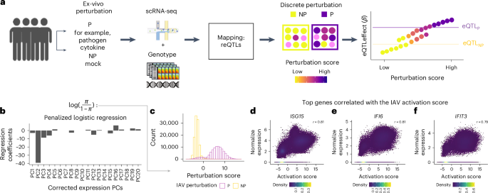
In contrast to traditional models that consider only the discrete perturbation state imposed by the experimental design, we define a continuous score to quantify the degree of perturbation response of each cell. The underlying assumption is that perturbation may induce changes in the transcriptional profile of a cell that are proportional to the degree of response of the cell. Similarly, experimental conditions may induce changes in the transcriptional profile of NP cells55,56,57,58,59. To systematically identify axes of variation in the transcriptional profile of P and NP cells, we use PCA and correct technical or biological effects with Harmony to obtain hPCs. We assume that one or several hPCs may capture the effect of perturbation in a cell.

To define a continuous perturbation score, we used a penalized logistic regression with hPCs as independent variables to predict the log odds of being in the pool of P cells, which serves as a surrogate of the cell’s degree of response to the experimental perturbation. Thus, for each perturbation model, we developed a continuous perturbation score of a cell by modeling the discrete perturbation state of a cell (i) (NP = 0, P = 1) as a function of the top 20 hPCs in a logistic Lasso regression model implemented in the R package glmnet60. We fitted the model and used the LASSO penalty term with a tuning parameter (λ) obtained from cross validation (cv.glmnet parameters: alpha = 1, lambda.1se)

$$\log \left(\frac{{\pi }_{i}}{1-{\pi }_{i}}\right)={\theta }_{i}+{\beta }_{\rm{PC}_{1}}{X}_{i,\rm{PC}_{1}}+\cdots +{\beta }_{\rm{PC}_{\textit{K}}}{X}_{i,\rm{PC}_{\textit{K}}}$$

(1)

where \(K\) is the number of PCs and πi is the probability of the cell (i) to be in the pool of P cells.

We use this approach instead of focusing on predefined gene sets such as the interferon-stimulated gene pathway for viral perturbations, which may not accurately represent the changes on the transcriptome in specific tissues, cells or perturbation experiments.

Cell-type-specific perturbation score

For each perturbation experiment, cell-type-specific perturbation scores for each main cell-type presented in PBMCs were generated by subsetting the dataset by cell-type and then performing the same steps as described before: gene normalization, scale, cosine normalization, selection of the 3,000 most variable genes (variance stabilizing transformation), PCA, harmony and Lasso regression using the top 20 corrected expression hPCs as predictors in the logistic Lasso regression model.

Correspondence of the perturbation score with canonical protein marker of response to perturbation

We evaluate the ability of the perturbation score generated using the penalized logistic regression to capture the response to perturbation. We re-analyzed a dataset of PBMCs perturbed with either anti CD3 and anti CD28 and LPS, which profiled cells using scRNA-seq as well as surface protein markers (CITE-seq)61. Thus, for each condition we calculated the perturbation score using the scRNA-seq data as described before. Then, we evaluate the Pearson correlation between the perturbation score of a cell and the expression of surface protein markers of activation.

Gene pathway enrichment analysis

For each perturbation experiment, we calculated the Pearson correlation between the 3,000 most variable genes and the perturbation score of a cell. We selected genes with a correlation Q < 0.05 (3,000 tests). Then, we used these correlation values to rank the genes and performed a gene pathway enrichment analysis using the fgsea R package27 with a maximum gene set size of 500, a minimum size of 15, and 100,000 permutations. We include the following gene sets from the Pathway Interaction Database stored in MSigDB: Hallmark gene set and large collection of immunological conditions (C7).

Prioritizing eQTLs in PBMCs bulk expression profiles

For each individual participant and perturbation condition, we summed the gene expression counts for each gene across all cells to generate bulk profiles, then we averaged the gene expression from each perturbation condition by individual participant, resulting in the average bulk expression profiles. This allows us to use a traditional eQTL linear regression model with one sample per donor to prioritize eQTLs. For each perturbation experiment, we generated bulk expression profiles for the NP, P and average conditions. We normalized the expression profiles (log2 count per million + 1) and applied an inverse rank normal transformation (qnorm((rank(gene, na.last = ‘keep’) − 0.5)/sum(!is.na(gene))). Then, we removed the effect of age, sex if available, top five genotype PCs and 15 latent factors using PEER factor analysis62. We only included transcripts expressed in at least 50% of the samples. The corrected gene expression was used as the dependent variable in our bulk cis-eQTL mapping. We performed the cis-eQTL mapping by testing each gene with genetic variants within 1 Mb of each gene’s transcription starting site using a linear regression implemented in FastQTL63. We use 1,000 permutations per locus and select the gene–SNP pairs (eGenes) with a Q value < 0.05. (Number of tests in IAV, 48,016,811; CA, 46,012,957; PA, 46,012,957; MTB, 44,896,173). In most cases, we prioritized the eQTL from the averaged NP and P profile as this produced the largest number of eQTLs (Q value < 0.10) (Supplementary Fig. 3). Standard approaches to fit the PME model are computationally expensive and impractical for the systematic genome-wide identification of eGenes in single-cell experiments.

Identifying response eQTL effects

For the single-cell approaches for both PBMCs or cell-type-specific analysis, we modeled the raw expression (E) counts in a cell (i) as a function of genotype allele dosage and an interaction with cell state accounting for confounders and technical batch using a described PME model18. For all the analyses, we included age and sex as fixed effects where available. We also controlled for genetic population stratification by including the top five genotype PCs (gPC) as covariates. Similarly, we controlled for unwanted variation in gene expression by including the top five gene expression PCs (ePC). In addition, we included the number of unique molecular identifier (UMIs) and percentage of reads mapping to mitochondrial genes (MT%) as fixed effects, and donor (d) and technical batch (b) as random effects. We include two cell state variables, the discrete perturbation state (Discrete: where P = 1 for perturbation or 0 for no perturbation) and the residual perturbation score (rScore) (3) that avoid the collinearity between the Discrete variable and the perturbation score (Score) from Eq. 1. To estimate the reQTL effect, we fit a model that included the genotype main effect (G) and the interaction terms of G with the Discrete (GxDiscrete) and rScore (GxrScore) variables. In contrast, we only included the interaction term GxDiscrete in the simplified 1df-discrete model. For the cell-type-specific reQTL analysis, we subset the dataset by each principal cell-type and used the cell-type-specific score and applied the same model (2) as described above.

$$\begin{array}{l}\log \left({E}_{i}\right)\;=\;\theta +{\beta }_{G}{X}_{d,{\rm{geno}}}+{\beta }_{{\rm{age}}}{X}_{d,{\rm{age}}}+{\beta }_{{\rm{nUMI}}}{X}_{i,{\rm{nUMI}}}+{\beta }_{{\rm{MT}}}{X}_{i,{\rm{MT}}}\\\qquad\qquad\;+{\beta }_{{\rm{Discrete}}}{X}_{i,{\rm{Discrete}}}+{\beta }_{{\rm{rScore}}}{X}_{i,{\rm{rScore}}}+{\beta }_{\rm{Gx}{\rm{rScore}}}{X}_{d,{\rm{geno}}}{X}_{i,{\rm{rScore}}}\\\qquad\quad\quad\;\,+{\beta }_{\rm{Gx}{\rm{Discrete}}}{X}_{d,{\rm{geno}}}{X}_{i,{\rm{Discrete}}}+\mathop{\sum}\limits_{k=1}^{5}{\beta }_{{g\rm{PC}}_{k}}{X}_{d,{g\rm{PC}}_{k}}\\\qquad\qquad\;+\mathop{\sum}\limits_{k=1}^{5}{\beta }_{{e\rm{PC}}_{k}}{X}_{i,{e\rm{PC}}_{k}}+\left(d\right)+({k}_{b}|b),\end{array}$$

(2)

$${\rm{Score}}=\theta +{\beta }_{{\rm{Discrete}}}{X}_{i,{\rm{Discrete}}}+{r\;\rm{Score}}.$$

(3)

To map reQTLs in bulk profiles (i) (Pseudobulk LME) we modeled the residuals from the PEER factor analysis (rPFA) as a function of the genotype and the GxDiscrete term accounting for donor’s age, sex and both the total numbers of UMIs and mean MT% across all cells per donor using an LME model. We included donor as a random effect in the LME model (equation (4)).

$$\begin{array}{l}{{\rm{rPFA}}}_{i}\;=\;\theta +{\beta }_{G}{X}_{d,{\rm{geno}}}+{\beta }_{{\rm{age}}}{X}_{d,{\rm{age}}}+{\beta}_{{\rm{nUMI}}}{X}_{i,{\rm{nUMI}}}+{\beta }_{{\rm{MT}}}{X}_{i,{\rm{MT}}}\\\qquad\qquad+{\beta }_{{\rm{Discrete}}}{X}_{i,{\rm{Discrete}}}+{\beta}_{{\rm{GxDiscrete}}}{X}_{d,{\rm{geno}}}{X}_{i,{\rm{Discrete}}}+\left(d\right)+\varepsilon .\end{array}$$

(4)

We compared the significance of each of these full models against a null model with no interaction terms using the likelihood ratio test and considered significant reQTLs to be those with an LRT Q value < 0.05. Furthermore, to rule out the possibility of spurious significant results, we performed 500 permutations per each discovered reQTL. For the permutation in the single-cell models, we shuffled values of the perturbation score and the discrete perturbation state randomly within each donor. For the pseudobulk LME model, we shuffled values of the perturbation state randomly across samples.

To exclude spurious associations, for each gene we counted the proportion of LRT P values from the permutation experiments that were smaller than the discovery LRT P (permutation P) and removed genes with permutation P < 0.05. To exclude genes where the PME model may not be appropriate due to high differential gene expression across cell states, we fit a PME model where we simulated null conditions by shuffling the perturbation score value randomly within each donor. We tested the significance of the interaction term under this null by comparing this model with a model with no GxScore term using the LRT ANOVA. For each eGene, we performed 100 permutations and removed eGenes where we observed a significant P value (LRT P < 0.01) in more than five out of 100 permutations.

In addition, we performed a secondary analysis for the CA, PA and MTB perturbation experiments based on the 1,825 eGenes prioritized by ref. 22 and listed in Supplementary Table 9 and passing QC in our preprocessing. For each perturbation experiment, we estimated reQTL effects for this set of 1,825 eQTLs using each of the models described above (equations (1) and (3)) and compared the significance against a null model with no interactions terms using the LRT and considered significant those with LRT Q value < 0.05. Furthermore, for each perturbation experiment, we generated P values under the uniform distribution based on the number of eQTLs included in our secondary analysis. Then, we calculated the enrichment of significant reQTLs in the 2df-model by comparing the number of tests where we found 2df-model LRT P < 0.001, >0.001 and ≤0.01, >0.01 and ≤0.05, >0.05 and ≤0.1, and >0.1 with those found under the uniform distribution using a χ2 test.

Estimating the eQTL effect at levels of the perturbation score

For any given reQTL, we selected cells either in the NP or P condition and calculated the 45th and 55th percentile of the perturbation score in that group. Then, we selected the cells with perturbation score values within the 45th to 55th percentile (50p) and estimated the eQTL effect in those cells by fitting a single-cell PME, where we modeled the raw gene counts (E) in a cell (i) as a function of the genotype (G) and the same cell and donor level fix and random covariates as described above (equation (2)) but without interaction terms (equation (5)). We consider the significance of the G term by comparing it with a null model with no G term using the LRT with 1 d.f.

$$\begin{array}{l}\log \left({E}_{i}\right)\;=\;\theta +{\beta }_{G}{X}_{d,{\rm{geno}}}+{\beta }_{{\rm{age}}}{X}_{d,{\rm{age}}}+{\beta }_{{\rm{nUMI}}}{X}_{i,{\rm{nUMI}}}+{\beta }_{{\rm{MT}}}{X}_{i,{\rm{MT}}}\\\qquad\qquad\quad+\mathop{\sum}\limits_{k=1}^{5}{\beta}_{{g\rm{PC}}_{k}}{X}_{d,{g\rm{PC}}_{k}}+\mathop{\sum}\limits_{k=1}^{5}{\beta }_{{e\rm{PC}}_{k}}{X}_{i,{e\rm{PC}}_{k}}+\left(d\right)+({k}_{b}|b).\end{array}$$

(5)

To visualize the eQTL effect at the donor level, we aggregated the gene counts in the cells in the 50p by donor and then normalized the gene expression (log2 counts per million + 1). Then, we plotted the gene expression as a function of the eQTL’s allele dosage.

Delta betas between PBMC and cell-type-specific reQTL analysis

First, based on the PBMCs analysis and for each main cell-type (that is, TCD4+, monocytes), we calculated the difference in the total eQTL between the 50th percentile in the P state versus the 50th percentile in the NP state (Delta 1). Furthermore, based on the cell-type-specific analysis (TCD4+ and TCD4+ perturbation score), we calculated the difference in the total eQTL between the 50th percentile in the P state versus the 50th percentile in the NP state (Delta 2). We only included eGenes with LRT Q value < 0.05 in the cell-type-specific analysis. Then, for each main cell-type we calculated the Pearson correlation between Delta 1 and Delta 2.

Composite eQTL effect in a cell

We defined the total eQTL in a cell (i) as the sum of the genotype main effect (G) with the discrete interaction effect (GxDiscrete) and the interaction effect with the residual of the perturbation score (GxrScore), weighted by its corresponding value (Discrete, NP = 0, P = 1; Score, continuous perturbation score) (Eq. 6).

$${{\beta }_{{\rm{total}}}=\beta }_{G}+{\beta }_{{\rm{GxDiscrete}}}{X}_{i}+{\beta }_{{\rm{GxrScore}}}{X}_{i}.$$

(6)

Comparison of the IAV perturbation score and an interferon-alpha score

As an alternative approach to quantify the response to perturbation, we developed a per cell interferon-alpha score based on a predefined gene set (MSigDB: Hallmark interferon-alpha response (INF-alpha))64. The selected genes (INF-alpha) were normalized, then we removed genes expressed in <1% of the cells and then scaled the expression of the gene (mean = 0, variance = 1). Then, for each cell, we averaged the expression across genes. To compare reQTL detected by each score, we ran a reduced single-cell reQTL model where we tested only for the significance of the interaction effect between the genotype and the score (GxScore). We then evaluated the number of significant reQTL (LRT Q value < 0.05) as well as the standardized effect size of the main eQTL effect (G) and interaction effects (GxScore) between the two approaches.

Comparison of Poisson mixed effect and negative binomial models

To confirm that the single-cell PME model was well calibrated, we fit a single-cell reQTL model where we modeled the raw expression counts in single cells as a function of genotype allele dosage and interaction terms equivalent to the PME 2df-model described in Eq. 1, using a negative binomial model implemented in the glmmTMB65 R package. We calculated the correlation between the LRT P value from the original PME and the negative binomial model.

Downsampling donors and cells

To test the effect of sample size on the power to detect reQTLs in the single-cell models, we generated datasets where we removed cells or removed donors randomly. We generated five datasets and, in each, we removed either 10, 20, 30, 40 or 50% of cells randomly within each donor. For each dataset, we generated three replicates by using different random seeds. Similarly, we generated five datasets with three replicates each where for each set we randomly removed either 10, 20, 30, 40 or 50% of donors. Then, in each downsampled dataset, we estimated reQTL effects with the PME model by testing the originally prioritized eGenes and counting the number of reQTLs that reached an LRT Q value < 0.05.

Power to detect reQTL at different degrees of perturbation

For each of the perturbation experiments (IAV, CA, PA and MTB), we generated three new datasets with different degrees of perturbation by sampling cells from the P condition (that is, cells exposed to IAV) at different ranges of the score (30th to 70th, 20th to 80th, and full distribution). We constrained the sampling so that each dataset contained the same number of P cells, and we kept all the NP cells. Then, we used the same set of prioritized eQTLs as the original analysis (IAV, 1,892; CA, 1,863; PA, 1,794; MTB, 1,355) and tested for reQTLs in single cells using both the 2df-model and the reduced 1df-discrete model. We compared the number of reQTLs that reached LRT Q value < 0.05 between the two models.

Similarly, for each perturbation experiment, we generated three additional new datasets by sampling P cells at different levels of the perturbation score (<33rd, >66th and the full distribution), again constraining the number of cells to be fixed between the datasets, and keeping all NP cells. We performed a reQTL analysis using both 2df-model and 1df-discrete models and compared the number of reQTLs that reached LRT Q value < 0.05 between the two models.

Comparison of the 2df-model with CellRegMap to find reQTLs in single cells

We compared our reQTL framework with CellRegMap19 (CRM), a statistical framework that can identify eQTLs with dynamic effects across cell-states in single cells. CRM can use PCs as cell states; however, in our comparison, we applied CRM using the residual effect of the perturbation score and the discrete perturbation state as these are the same cell-states used in our 2df-model. In the CA perturbation experiment, we defined a set of ground-truth reQTLs. These were reQTLs detected by the original analysis by Oelen et al.22 and detected in our pseudobulk reQTL approach. Similarly, we defined a set of negative controls as those reQTLs not reported by Oelen et al.22 or our pseudobulk analysis (LRT Q value > 0.2). In addition, for every ground-true reQTL, we randomly selected three negative controls with mean gene expression within the range of the mean gene expression of positive control ± (mean positive/2). Based on these criteria, we had 35 positive reQTL and 105 negative controls, and we tested for reQTLs using our 2df-model and CRM with the default parameters. We corrected for multiple comparisons using a Bonferroni correction and compared the sensitivity and specificity of the two models.

reQTLs with heterogeneous effects across cell types

We tested for heterogeneous effects by comparing the effect size of each of the interaction terms between cell types. For each perturbation experiment, we selected cells from each main cell type present in the experiment (IAV: B, CD4+ T, CD8+ T, Monocytes, NK; CA-PA-MTB: B, CD4+ T, CD8+ T, Monocytes, NK, DC) and fitted the single-cell 2df-model with the GxDiscrete and GxScore terms. Then, for each reQTL, we used the summary statistics to compare the effect sizes of each of the interaction’s terms across cell types. We tested whether the variability in the observed effect sizes is larger than the expected based on sampling variability alone using the Cochran’s Q test (Q) implemented in the metafor R package (rma, method = ‘FE,’ weighted = TRUE). We defined response eQTLs with heterogeneous effects as those with a Cochrane’s Q-test Q value < 0.10 in at least one of the interaction terms.

$$\begin{array}{ccc}{\beta }_{{\rm{meta}}}=\left(\mathop{\sum }\limits_{k=1}^{K}\frac{{\beta }_{k}}{s{{e}_{k}}^{2}}\right)\left/\left(\mathop{\sum }\limits_{k=1}^{K}\frac{1}{s{{e}_{k}}^{2}}\right)\right.&{\rm{and}}& Q=\mathop{\sum }\limits_{k=1}^{K}\frac{1}{s{{e}_{k}}^{2}}{\left({\beta }_{k}-{\beta}_{{\rm{meta}}}\right)}^{2}\end{array},$$

where \(K\) is the number of cell types in the perturbation experiment, \({\beta }_{k}\) is the effect size for each cell-type, and \({\beta }_{{\rm{meta}}}\) is the average effect size weighted by the inverse of the variance of the estimate on each cell type.

Overlap with previous response eQTLs in response to IAV

We compared the overlap between the reQTLs found in the IAV dataset using the 2df-model (all PBMCs and monocyte-specific) and the reQTLs found after IAV perturbation in primary monocytes reported originally in Table S2 by Quach et al.29. There were 286 eGenes present in both analyses. We compared the overlap of eGenes with significant reQTLs (LRT Q value < 0.05) found in our PBMC analysis and the monocyte-specific analysis of the IAV dataset. Similarly, we selected eGenes with reported reQTLs P value from Quach et al.29. In the case of several reQTLs per gene reported in ref. 29, we chose the result with the lowest reQTL P value.

Colocalization analysis

To find instances where a perturbation-dependent reQTL shared its causal variant with a GWAS locus, we performed a colocalization analysis using coloc66 (coloc.abf), a Bayesian approach that estimates the posterior probability of having a shared true causal variant between the eQTL and the GWAS locus. We used summary statistics from nine GWAS on immune traits (type 1 diabetes67, multiple sclerosis68, asthma69, RA1, SLE33, inflammatory bowel disease70, Crohn’s disease70, ulcerative colitis70, psoriasis71) and three GWAS on nonimmune traits (coronary artery disease72, type 2 diabetes73, depression74).

We defined eQTLs as those with a nominal Q value < 0.05 in the analysis with FastQTL. We ran coloc with the default parameters and defined colocalization as those loci with a posterior probability H4 (PPH4) > 0.5. Furthermore, for those colocalized loci, we generated the 95% credible set and obtained the posterior probability of each variant within the credible set (snpH4) under the single causal variant assumption. We calculated the enrichment of colocalization in eGenes with reQTL effect compared to eGenes with no reQTL effect using Fisher’s exact test.

In addition, to find colocalization at different levels of the perturbation score, we defined tertiles of perturbation within the NP (T1–T3) and P (T4–T6) conditions. For example, in the IAV experiment, T1 was defined as NP cells with perturbation score values <33rd percentile (−0.90), T2 was defined as NP cells with the perturbation score ≥33rd and below 66th percentile (−0.75) and T3 was defined as NP cells with a perturbation score ≥ 66th percentile. Then, for each tertile, we generated pseudobulk gene expression profiles, tested for cis-eQTL and ran coloc as described before.

Reporting summary

Further information on research design is available in the Nature Portfolio Reporting Summary linked to this article.