
Input embeddings
In CellNavi, we use single-cell raw count matrices as the only input. Specifically, the single-cell sequencing data are processed into a cell-by-gene count matrix, \({\bf{X}}\in {{\mathbb{R}}}^{N\times G}\), where each element \({{\bf{X}}}_{n,g}\) represents the expression of the nth cell and the gth gene (or read count of the gth RNA).
To better describe a gene’s state in a cell, we involve both gene name and gene expression information in its input embeddings. Formally, the input embedding of a token is the concatenation of gene name embedding and gene expression embedding.
Gene name embedding
We use a learnable gene name embedding in CellNavi. The vocabulary of genes is obtained by taking the union set of gene names among all datasets. Then, the integer identifier of each gene in the vocabulary is fed into an embedding layer to obtain its gene name embedding. In addition, we incorporate a special token \({\rm{CLS}}\) in the vocabulary for aggregating all genes into a cell representation. The gene name embedding of cell \(n\) can be represented as \({{\bf{h}}}_{n}^{({\rm{name}})}\in {{\mathbb{R}}}^{(G+1)\times H}\):
$$\,{{\bf{h}}}_{n}^{({\rm{name}})}=\left[{{\bf{h}}}_{n,{\rm{CLS}}}^{\left({\rm{name}}\right)},\,{{\bf{h}}}_{n,\,1}^{\left({\rm{name}}\right)},\,{{\bf{h}}}_{n,\,2}^{\left({\rm{name}}\right)},\ldots ,\,{{\bf{h}}}_{n,G}^{\left({\rm{name}}\right)}\right],$$
where \(H\) is the dimension of embeddings, which is set to 256.
Gene expression embedding
One major challenge in modelling gene expression is the variability in absolute magnitudes across different sequencing protocols13. We tackled this challenge by normalizing the raw count expression for each cell using the shifted logarithm, which is defined as
$${\widetilde{{\bf{X}}}}_{n,g}=\log \left(L\frac{{{\bf{X}}}_{n,g}}{\sum _{{g}^{{\prime} }}{{\bf{X}}}_{n,{g}^{{\prime} }}}+1\right),$$
where \({{\bf{X}}}_{n,g}\) is the raw count of gene \(g\) in cell \(n\), \(L\) is a scaling factor and we used a fixed value \({L}={1\times 10}^{4}\) in this study, and \({\widetilde{{\bf{X}}}}_{n,g}\) denotes the normalized count. Finally, a linear layer was applied on the normalized expression \({\widetilde{{\bf{X}}}}_{n,g}\) to obtain the gene expression embedding. For the \({\rm{CLS}}\) token, we set it as a unique value for gene expression embedding. The gene expression embedding of cell \(n\) can be represented as \({{\bf{h}}}_{n}^{({\rm{expr}})}\in {{\mathbb{R}}}^{(G+1)\times H}\):
$${{\bf{h}}}_{n}^{({\rm{expr}})}=\left[{{\bf{h}}}_{n,{\rm{CLS}}}^{\left({\rm{expr}}\right)},\,{{\bf{h}}}_{n,1}^{\left({\rm{expr}}\right)},\,{{\bf{h}}}_{n,2}^{\left({\rm{expr}}\right)},\ldots ,\,{{\bf{h}}}_{n,G}^{\left({\rm{expr}}\right)}\right].$$
The final embedding of cell \(n\) is defined as the concatenation of \({{\bf{h}}}_{n}^{({\rm{name}})}\) and \({{\bf{h}}}_{n}^{({\rm{expr}})}\):
$${{\bf{h}}}_{n}={\rm{SUM}}\left({{\bf{h}}}_{n}^{\left({\rm{name}}\right)},\,{{\bf{h}}}_{n}^{\left({\rm{expr}}\right)}\right)\in {{\mathbb{R}}}^{\left(G+1\right)\times H}.$$
Cell manifold modelModel architecture
The CMM, is composed of six layers of a transformer variant that is designed specifically for processing graph-structured data (GeneGraph attention layers)19. The encoder takes the input embeddings to generate cell representations and uses only genes with non-zero expressions. To further speed up training, also as an approach of data augmentation, we performed a gene sampling strategy by randomly selecting at most 2,048 genes as input. It should be noted that the strategy is applied only during training; all non-zero genes are included at inference stage to avoid information loss. We use \({{\bf{h}}}_{n}^{(l)}\) to represent the embedding of cell n at the lth layer, where \({{\bf{h}}}_{n}^{(l)}\) is defined as
$${{\bf{h}}}_{n}^{(l)}=\left\{\begin{array}{c}{{\bf{h}}}_{n},\,l=0,\\ {\rm{GeneGraphAttnLayer}}\left({{\bf{h}}}_{n}^{\left(l-1\right)}\right),l\in \left[1,6\right].\end{array}\right.$$
The multihead attention module in each GeneGraph attention layer consists of three components. In addition to a self-attention module, a centrality encoding module and a spatial encoding module are also incorporated to modify the standard self-attention module for graph data integration.
We start by introducing the standard self-attention module. Let \({N}_{{\rm{heads}}}\) be the number of heads in the self-attention module. In the lth layer, ith head, self-attention is calculated as
$$\begin{array}{c}{{\bf{Q}}}_{n}^{(l,i)}={{\bf{h}}}_{n}^{(l)}{{\bf{W}}}^{({\rm{qry}},i)},{{\bf{K}}}_{n}^{(l,i)}={{\bf{h}}}_{n}^{(l)}{{\bf{W}}}^{({\rm{key}},i)},{{\bf{V}}}_{n}^{(l,i)}={{\bf{h}}}_{n}^{(l)}{{\bf{W}}}^{({\rm{val}},i)},\\ {{\bf{A}}}_{n}^{(l,i)}=\frac{{{\bf{Q}}}_{n}^{(l,i)}{\left({{\bf{K}}}_{n}^{(l,i)}\right)}^{\top }}{\sqrt{D}},{\rm{Attn}}\frac{(l,i)}{n}={\rm{softmax}}\left({{\bf{A}}}_{n}^{(l,i)}\right){{\bf{V}}}_{n}^{(l,i)},\\ {{\bf{h}}}_{n}^{(l){\prime} }={\rm{CONCAT}}\left({{\rm{Attn}}}_{n}^{(l,1)},\cdots ,{{\rm{Attn}}}_{n}^{(l,{N}_{{\rm{heads}}})}\right){{\bf{W}}}^{({\rm{out}})}\in {{\mathbb{R}}}^{(G+1)\times 2H},\end{array}$$
where \({{\bf{W}}}^{\left({\rm{qry}},{i}\right)}\), \({{\bf{W}}}^{\left({\rm{key}},i\right)}\) and \({{\bf{W}}}^{\left({\rm{val}},i\right)}\in {{\mathbb{R}}}^{2H\times D}\) are learnable matrices that project input embedding \({{\bf{h}}}_{n}^{\left(l\right)}\) of cell \(n\) in to \({{\bf{Q}}}_{n}^{\left(l,i\right)}\),\(\,{{\bf{K}}}_{n}^{\left(l,i\right)}\) and \({{\bf{V}}}_{n}^{\left(l,i\right)}\), the symbol \({{\bf{W}}}^{({\rm{out}})}\in {{\mathbb{R}}}^{\left(D{N}_{{\rm{heads}}}\right)\times 2H}\) is a learnable linear projection that refines the output of multihead attention, and D is the feature dimension for each attention head that satisfies DNheads = 2H. The output of multihead attention \({{{\bf{h}}}_{{\rm{n}}}^{\left(l\right)}}^{{\prime} }\) is then passed through a layer normalization layer and a multilayer perceptron (MLP) model, producing the final output \({{\bf{h}}}_{n}^{(l+1)}\) as the input to the next layer.
The standard attention mechanism processes features of each individual gene independently, whereas the gene graph incorporates relational information between genes. To incorporate the gene graph information into the model, the centrality encoding module projects the relational information into the regulatory activity feature of each single gene, and the spatial encoding module directly incorporates the relational information with the attention mechanism. More specifically, we define \({{\bf{z}}}_{{{\rm{deg}}}^{-}({\mathcal{G}},g)}^{-}\) and \({{\bf{z}}}_{{{\rm{deg}}}^{+}({\mathcal{G}},g)}^{+}\), learnable embeddings describing in-degree deg− and out-degree deg+ of gene g on the gene graph \({\mathcal{G}}\). We add these embeddings to the gene embeddings to update cell encoding:
$${{\bf{h}}}_{n,g}^{(l)}={{\bf{h}}}_{n,g}^{(l){\prime}}+{{\bf{z}}}_{{{\rm{deg}}}^{-}({\mathcal{G}},g)}^{-}+{{\bf{z}}}_{{{\rm{deg}}}^{+}({\mathcal{G}},g)}^{+}.$$
This cell encoding update by the centrality encoding module is applied before the self-attention module.
The spatial encoding module aims to capture regulation relations between genes from the gene graph. For this purpose, we generate the distance matrix \({\bf{S}}\in {{\mathbb{N}}}^{G\times G}\), which contains the shortest distances between gene pairs on the gene graph \({\mathscr{G}}\). We assign each element in \({\bf{S}}\) as a learnable bias added to attention weights:
$${{\bf{A}}}_{{g}_{1},{g}_{2}}^{{\prime} }={{\bf{A}}}_{{g}_{1},{g}_{2}}+b\left({{\bf{S}}}_{{g}_{1},{g}_{2}}\right),$$
where \(b\) is a learnable scalar-valued function of the distance \(\,{{\bf{S}}}_{{g}_{1},{g}_{2}}\). It assigns a special value to genes that are not connected to the graph. We use \({{\bf{A}}}^{{\prime} }\) in place of the original attention weights \({\bf{A}}\) in the standard self-attention module when computing self-attention in our model. In our implementation, we apply layer normalization and an MLP before computing multihead self-attention. The cell representation output from the CMM, \({{\bf{h}}}_{n,{\rm{CLS}}}^{(6)}\), is subsequently passed through a fully connected layer, where the dimensionality is increased from 256 to 2,048. This resulting value serves as the cell coordinate for cell \(n\), denoted as \({{\bf{CRD}}}_{n}\).
CMM pretraining task
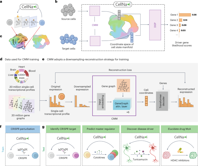
The CMM is expected to generate cell coordinates that parameterize the intrinsic features and variables (that are much less than the dimensions in the raw gene expression profile representation) of a cell state and maintain cell similarity in the vector space, to provide a concise and biologically relevant representation for the DGP to consume. To achieve this, we design a downsampling reconstruction pretraining task, which asks the CMM to produce a cell coordinates of a downsampled gene expression \({{\bf{X}}}_{n}^{\left({\rm{ds}}\right)}\) of a cell \(n\), that allows a separate decoder model to reconstruct the original gene expression \({{\bf{X}}}_{n}\) of that cell as accurate as possible. To achieve this, the CMM is enforced to capture the co-varying patterns among the raw gene expression dimensions, hence helping the CMM to extract the underlying intrinsic variables.
Specifically, for the downsampling process, we downsample the raw count expression of each gene via a binomial distribution. The downsampled expression \({{\bf{X}}}_{n,g}^{({\rm{ds}})}\) of the nth cell and the gth gene is produced by
$${{\bf{X}}}_{n,g}^{\left({\rm{ds}}\right)}\sim B\left({{\bf{X}}}_{n,g},\frac{1}{{r}^{\;\left({\rm{ds}}\right)}}\right),$$
where the ∼ denotes ‘is distributed as’, \({{\bf{X}}}_{n,g}\) is the raw count of gene \(g\) in cell \(n\), \({r}^{\;\left({\rm{ds}}\right)}\) is the downsample rate that is uniformly sampled from \([1,\,20)\), and \(B\) denotes the binomial distribution. The decoder is an MLP consisting of two linear layers. For each downsampled gene expression, the decoder concatenates the cell coordinates \({{\bf{CRD}}}_{n}\) of \({{\bf{X}}}_{n}^{\left({\rm{ds}}\right)}\) produced by the CMM and the embedding of that gene as the direct input to the MLP. The MLP output comes in the same shape as \({{\bf{X}}}_{n}\).
The learning objective for reconstructing the original gene expression profile \({{\bf{X}}}_{n}\) from the downsampled version \({{\bf{X}}}_{n}^{\left({\rm{ds}}\right)}\) is
$${ {\mathcal L} }_{{\rm{recons}}}=\frac{1}{N}\mathop{\sum }\limits_{n=1}^{N}{\Vert {\rm{DEC}}\left({\bf{C}}{\bf{R}}{\bf{D}}\left({{\bf{X}}}_{n}^{({\rm{ds}})}\right)\right)-{{\bf{X}}}_{n}\Vert }^{2},$$
where \(\,{\|\cdot \|}^{2}\) represents the squared 2-norm of a vector. Both the CMM and the decoder are optimized. After pretraining, the CMM is to be used for driver gene prediction, while the decoder is discarded.
Driver gene predictor
The driver gene classifier is an MLP consisting of two linear layers. It is optimized to predict the perturbed genes from a pair of cell coordinates output by the CMM. To be more specific, transcriptomes of source cell \({{\bf{X}}}_{{\rm{src}}}\) and target cell \({{\bf{X}}}_{{\rm{tgt}}}\) are mapped to cell coordinates \({{\bf{CRD}}}_{{\rm{src}}}\) and \({{\bf{CRD}}}_{{\rm{tgt}}}\) with the CMM. For the direct input features, the DGP concatenates the two cell coordinates and then proceeds with an MLP, which outputs the logits of genes. We use the cross-entropy loss for training the DGP:
$${{\mathscr{L}}}_{{\rm{driver\_gene}}}={\rm{CE}}\left({\rm{DGP}}\left({\rm{CONCAT}}\left({\bf{CRD}}\left({{\bf{X}}}_{{\rm{src}}}\right),{\bf{CRD}}\left({{\bf{X}}}_{{\rm{tgt}}}\right)\right)\right),{g}_{{\rm{drv}}}\right),$$
where \({\rm{CE}}\left({\bf{l}},g\right)=\frac{{{\bf{l}}}_{g}}{\log {\sum }_{{g}^{{\prime} }}\exp \left({{\bf{l}}}_{{g}^{{\prime} }}\right)}\) is the cross-entropy loss, and \({g}_{{\rm{drv}}}\) denotes the driver gene corresponding to \({{\bf{X}}}_{{\rm{src}}}\) and \({{\bf{X}}}_{{\rm{tgt}}}\). The loss is finally averaged over all \(\left({{\bf{X}}}_{{\rm{src}}},{{\bf{X}}}_{{\rm{tgt}}},{g}_{{\rm{drv}}}\right)\) tuples in the dataset. The pretrained CMM used to produce \({{\bf{CRD}}}_{{\rm{src}}}\) and \({{\bf{CRD}}}_{{\rm{tgt}}}\) is also fine-tuned together with the DGP by this loss.
Additional training details for CellNavi are available in Supplementary Note 4.
BaselinesSCENIC and SCENIC+
For each test dataset, SCENIC+ inferred a GRN, identified regulons \({{\bf{W}}}_{r}\in {{\mathbb{R}}}^{{N}_{r}\times {N}_{g}}\), and computed regulon activity \({{\bf{W}}}_{a}\in {{\mathbb{R}}}^{{N}_{c}\times {N}_{r}}\) in the cells, where \({N}_{r},\,{N}_{g}\,\text{and}\,{N}_{c}\) represent the number of identified regulons, genes and cells in the test dataset, respectively. \({{\bf{W}}}_{r}\) is a learnt matrix containing the weights of genes for different regulons, and \({{\bf{W}}}_{a}\) indicates the regulon activities for each cell. Then, we used \({{\bf{W}}}_{g}={{\bf{W}}}_{a}{{\bf{W}}}_{r}\) to represent the regulatory importance of each gene in cells. Based on these values (elements in \({{\bf{W}}}_{g}\)), genes in each cell were ranked, with higher values indicating a greater potential role in controlling cellular identity. We applied SCENIC+ to Norman et al. and Schmidt et al. datasets. Only genes present in the perturbation pools of these datasets were included in the ranking based on \({W}_{g}\). Hyperparameters of GRN inference, regulon identification and regulon activation were set to default. Cells with no regulon activated were removed from our analysis. SCENIC+ analysis was realized by pyscenic 0.12.1.
Other GRNs
We constructed GRNs using three alternative methods: GRNBoost2, GENIE3 and RENGE, following default parameters from prior studies where applicable. Due to computational memory constraints, we limited the analysis for GENIE3 and RENGE to the top 5,000 highly variable genes. For GENIE3 and GRNBoost2, we utilized the SCENIC implementation to infer GRNs. For RENGE, which is designed to infer GRNs using time-series single-cell RNA sequencing (RNA-seq) data, we adapted the method to work with static single-cell RNA-seq data. After constructing GRNs with these methods, we applied the same downstream analysis protocol as described for the SCENIC pipeline.
In silico perturbation
In silico perturbation methods, such as GEARS, are capable of predicting transcriptomic outcomes of genetic perturbations. We trained GEARS model on the datasets mentioned in the corresponding tasks. For evaluation, we computed the cosine similarity between the predicted transcriptomic profiles under various perturbations and the corresponding profiles of cells from the test datasets. Driver genes were predicted on the basis of the similarities, and high values in similarity indicate the potential to be driver genes. GEARS analysis was realized by cell-gears 0.1.1. Data processing and training followed the data processing tutorial (https://github.com/snap-stanford/GEARS/blob/master/demo/data_tutorial.ipynb) and training tutorials (https://github.com/snap-stanford/GEARS/blob/master/demo/model_tutorial.ipynb).
DGE analysis
DGE analysis is the most frequently used method to reveal cell-type-specific transcriptomic signature. Initially, cells from the test datasets were normalized and subjected to logarithmic transformation. Subsequently, we applied the Leiden algorithm, an unsupervised clustering method, to categorize the target cells into distinct groups. The number of clusters for each test dataset was set to range from 20 to 40, ensuring that cellular heterogeneity was maintained while providing a sufficient number of cells in each group for robust statistical analysis. We selected source cells to serve as a reference for comparison and performed DGE analysis on each target cell group against this reference. The Wilcoxon signed-rank test was used to determine statistical significance. Then, significant genes were ranked according to their log-fold changes in expression as potential driver genes. Both unsupervised clustering and DGE analysis were conducted using the package scanpy 1.9.6.
The prior gene graph
The prior gene graph was constructed from NicheNet, where GRN and cellular signalling network were integrated. The gene graph is a directional graph. More specifically, for each gene node on the graph, the number of incoming edges corresponds to the genes that regulate it, while the number of outgoing edges represents the genes it regulates. In our approach, a connection was established between two genes if they were linked in either of the individual networks. The resulting integrated graph features 33,354 genes, each represented by a unique human gene symbol, and includes 8,452,360 edges that signify the potential interactions. The unweighted versions of NicheNet networks were used in our approach. For each cell, we remove the gene nodes with values of 0 in the raw count matrix of the single-cell transcriptomic profile, to construct the cell-type-specific gene graph. During pretraining, when downsampling is performed on single-cell transcriptomes, only the non-zero genes included as model input are retained to generate sample-specific graphs that guide the model’s task.
To evaluate the impact of graph connectivity and structure, we generated alternative graph configurations as follows:
(1)
Fully connected graph: A maximally connected graph where every pair of genes is connected by an edge of equal weight.
(2)
Sparsified graphs: Graphs were created by downsampling the total number of edges from the original graph to 1/10 and 1/20 of its total edges, enabling an evaluation of how reduced connectivity affects performance.
(3)
Random graphs: Randomized graphs were generated while preserving the number of nodes and certain structural properties of the original graph, such as self-loops. Edges were introduced probabilistically to maintain overall consistency with the original graph’s sparsity and connectivity.
DatasetsHuman Cell Atlas
We downloaded all single-cell and single-nucleus datasets sourced from contributors or DCP/2 analysis in Homo sapiens up to March 2023, accumulating approximately 1.5 TB of raw data. We retained all experiments that included raw count matrices and standardized the variables to gene names using a mapping list obtained from Ensembl (https://www.ensembl.org/biomart/martview/574df5074dc07f2ee092b52c276ca4fc).
Norman et al
This dataset (GSE133344) measures transcriptomic consequences of CRISPR-mediated gene activation perturbations in K562 cell line. We filtered this dataset by removing cells with a total count below 3,500. After filtering, this dataset contained 105 perturbations targeting different genes, and 131 double perturbations targeting two genes simultaneously. We used unperturbed cells (with non-targeting guide RNA) as source cells and perturbed cells as target cells.
Schmidt et al
This dataset (GSE190604) measures the effects of CRISPR-mediated activation perturbations in human primary T cells under both stimulated and resting conditions. For our analysis, we excluded cells not mentioned in metadata and removed genes appeared in less than 50 cells. Gene expression levels of single guide RNA were deleted to avoid data leakage. We used unperturbed cells as source cells and perturbed cells as target cells. We also excluded cells without significant changes after perturbation following the procedure proposed by Mixscape tutorial via package pertpy. Default parameters were used for Mixscape analysis.
Cano-Gamez et al
This dataset (EGAS00001003215) comprises naive and memory T cells induced by several sets of cytokines. With cytokine stimulation, T cells are expected to differentiate into different subtypes. We took cells not treated by cytokines as source cells and cytokine-stimulated cells as target cells. This experimental set reflects the differential process of human T cells. For our analysis, clusters 14–17 were excluded because their source cells could not be reliably determined.
Fernandes et al
This dataset comprises heterogeneous dopamine neurons derived from human iPS cells. These neurons were exposed to oxidative stress and ER stress, representing PD-like phenotypes. We followed preprocessing procedures as mentioned in the original GitHub repo (https://github.com/metzakopian-lab/DNscRNAseq/blob/master/preprocessing.ipynb).
Tian et al
This dataset comprises iPS cell-derived neurons perturbed by more than 180 genes related to neurodegenerative diseases. CRISPR interference experiments with single-cell transcriptomic readouts were conducted by CRISPR droplet sequencing (CROP-seq). For our analysis, we removed genes that appeared in fewer than 50 cells. We used unperturbed cells as source cells and perturbed cells as target cells.
Srivatsan et al
This dataset (GSE139944) contains transcriptomic profiles of human cell lines perturbed by compounds. For our study, we utilized K562 cell line cells perturbed by HDAC inhibitors. We used unperturbed cells as source cells, and chemically perturbed cells as target cells. This set represents the process of cellular transition caused by drugs.
Kowalski et al
This dataset (GEO: GSE269600) measures the transcriptional consequences of CRISPR-mediated perturbations in HEK293FT and K562 cells. For our analysis, we excluded perturbations that consisted of fewer than 200 cells. Cells with minimal perturbation effects were removed from downstream analysis. We used cells from control groups as source cells, and perturbed cells as target cells.
T cell differentiation analysisIdentification of cellular phenotypic shift
We computed the transition score to identify cellular phenotypic shifts on the transcriptomic level. We selected canonical marker genes associated with IFNG and IL2 secretion and Th2 differentiation. Then, we computed the transition score based on the mean expression level of these marker genes, that is, \({\rm{CT}}{{\rm{S}}}_{{ij}}=\frac{1}{{K}_{i}}\mathop{\sum }\nolimits_{{k}_{i}=1}^{{K}_{i}}({g}_{{j}_{1}{k}_{i}}-{g}_{{j}_{0}{k}_{i}})\), where \({\rm{CT}}{{\rm{S}}}_{{ij}}\) is the transition score of phenotypic shift type i in source–target cell pair \(j\), \({g}_{{j}_{1}{k}_{i}}\) and \({g}_{{j}_{0}{k}_{i}}\) are normalized gene expression levels of marker gene k for cell-state transition type i in target cell j1 and its source cell j0. The total number of marker genes for phenotypic shift type i is represented with Ki. Then, classes of phenotypic changes were annotated on the basis of transition score. Transition scores are calculated via function tl.score_genes from scanpy package with default parameters.
Cell type classification with predicted driver genes
We selected a series of genes related to transition mentioned above from previous studies (Supplementary Table 4). We used the term ‘likelihood scores’ to describe the probability of a gene to be a driver factor predicted by the model, that is,
$${{\rm{LS}}}_{{jk}}^{\mathrm{mod}}={p}_{{jk}}^{\mathrm{mod}},$$
where \({{\rm{LS}}}_{{jk}}^{\mathrm{mod}}\) means the likelihood score for gene \(k\) in source–target cell pair \(j\) from model \(\mathrm{mod}\), and \({p}_{{jk}}^{\mathrm{mod}}\) represents the probability predicted by model \(\mathrm{mod}\). For our analysis, the \(\mathrm{mod}\) could be CellNavi, or baseline models.
Then, we aggregate likelihood scores into ‘prediction scores’ to evaluate the performance of different models:
$${{\rm{PS}}}_{{ij}}^{\mathrm{mod}}=\frac{1}{{m}_{i}}\mathop{\sum }\limits_{{k}_{i}=1}^{{m}_{i}}{{\rm{LS}}}_{{jk}}^{\mathrm{mod}},$$
where \({{\rm{PS}}}_{{ij}}^{\mathrm{mod}}\) is the prediction score of cell-state transition type i in source–target cell pair j predicted by model mod. The number of candidate driver genes for each phenotypic changing type i is mi. Ideal prediction should reflect similar patterns as shown by the cellular transition score mentioned above. To evaluate it quantitatively, we trained decision tree classifiers with prediction scores as input to test whether predictions scores would faithfully demonstrate cell-state transition types. Classifiers were trained for each method independently, and tenfold cross-validation was conducted. Classifiers were implemented via shallow decision trees using the sklearn package.
GO enrichment analysis
We used GO enrichment analysis to explore drugs’ mechanisms of action. For each drug compound, the top 50 genes with highest scores predicted by CellNavi were used for GO enrichment analysis. The significant level was chosen to be 0.05, and the Benjamini–Hochberg procedure was used to control the false discovery rate. For implementation, we used package goatools for GO enrichment analysis.
Molecular docking
We performed molecular docking for panobinostat and tucidinostat, with a reference protein structure obtained from the PDB entry 3MAX. The ligand structures from PDB entries 3MAX and 5G3W were used to guide the initial placement of panobinostat and tucidinostat, ensuring the pose correctness of the warheads and major scaffolds. Based on such initial poses, local optimizations were performed with AutoDock Vina. PyMol was used for structure visualization.
Reporting summary
Further information on research design is available in the Nature Portfolio Reporting Summary linked to this article.