
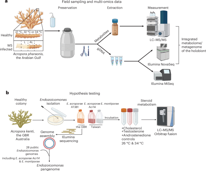
Sampling
Samples were collected at Saadiyat Reef, Abu Dhabi, UAE (24° 35’ 54.2’ N, 54° 25’ 12.9’ E) by SCUBA at a depth of 6–7 m from Acropora pharaonis corals26,54. Colonies were monitored for 6 months before sampling started in June, August and October 2016. Environmental parameters (GPS coordinates, temperature, salinity, pH, dissolved oxygen, turbidity and redox potential) were measured in situ with a YSI Multimeter on each sampling day (Extended Data Table 1). Nubbins of ~5 cm length were cut off with a garden shear and transferred to sterile ziplock bags filled with surrounding seawater. On the surface, nubbins were removed from the bag, placed on aluminum foil, washed for a few seconds with a small amount of sterile MilliQ-H2O to remove excess seawater, wrapped and flash frozen in liquid nitrogen. The samples were stored at −80 °C until further processing. While morphological characteristics were used for coral taxonomy in this study, molecular approaches can further refine species identification amid ongoing taxonomic uncertainties.
DNA extraction
Using bleach-cleaned scissors and forceps, each coral fragment (~0.5 cm2) was placed on dry ice, rinsed thoroughly with MilliQ-H2O, gently dried and placed at the bottom of a 2.0 ml reinforced tube kept on ice. Two 3-mm stainless steel beads (acid-cleaned and sterilized) were added. Samples were incubated at 65 °C for 30 min with 1 µl of RNase, Proteinase K (Promega) (1 mg ml−1 in MilliQ-H2O), lysozyme (1 mg ml−1 in MilliQ-H2O) (Sigma) and 600 µl Qiagen kit lysis buffer. Samples were homogenized twice for 10 min at medium speed with a Tissuelyzer (Qiagen). Cell debris/coral skeleton was removed by centrifugation at 18,000 g for 10 min in a 5430 microcentrifuge (Eppendorf) at room temperature. The resulting supernatant was transferred to a fresh sterile low-bind microcentrifuge tube (Eppendorf) and DNA purified using the Qiagen All-prep-kit (Qiagen) according to manufacturer instructions. DNA was further purified using magnetic beads (AMPure XP system) with two sequential ethanol washing steps.
16S rRNA gene amplicon sequencing
DNA samples were prepared at 10–50 ng µl−1 according to Qubit 2.0 (ThermoFisher) measurements and were delivered on dry ice to the Carver Biotechnology Center (University of Illinois-Urbana Champagne, Champaign and Urbana, IL, USA) for sequencing. Briefly, libraries were prepared with the hypervariable region V4 515 F GTGYCAGCMGCCGCGGTAA and V4 806 R GGACTACNVGGGTWTCTAAT primer pair for bacterial 16S rRNA gene amplification55,56, with spiked PhiX as the positive control, and sequenced with MiSeq 2 × 250 (Illumina). Sequencing yielded 22 samples with sufficient reads after FASTQ checking and trimming were completed. Sequences were analysed using DADA2 (v.3.6.0)57 in R. The DADA2 R-script uses raw amplicon sequencing data in FASTQ format as input. Error correction of the reads was performed, where reads were quality filtered, dereplicated, chimaeras were removed, and end pairs were merged to infer amplicon sequence variants (ASVs). For taxonomic assignment of the ASVs, the sequences were aligned against the SILVA database (release 132)58. Chloroplasts, mitochondria and eukaryotic reads were removed. An average of 6,972 reads per sample was obtained. The ASV data were then processed using the rANOMALY R package59. Beta diversity was assessed and visualized through principal coordinates analysis (PCoA) based on pairwise Bray–Curtis distances and tested using PERMANOVA. All plots were generated using the ggplot60 and phyloseq61 R packages, and all statistical analyses were conducted in R v.4.1.1.
Shotgun metagenomic sequencing
DNA samples were prepared following the NovoSeq Nano DNA Sample Preparation Guide. Sequencing was performed using an Illumina Novoseq 6000 (Illumina) with 2 × 150 bp read length at Novogene. A total of 14 metagenomic libraries (3 replicates × 5 conditions) were prepared at 50 ng ml−1 concentration. Only one sample was not sequenced for the 27 °C condition due to an inadequate amount of gDNA. Sequencing produced a total of 590 Gb of data (on average, 42 Gb per sample) and on average, 280 million paired-end (PE) reads per sample (Supplementary Table 3).
Quality control and in silico partitioning of coral holobiont metagenomes
Illumina reads were checked for quality using fastqc v.0.11.9 (https://www.bioinformatics.babraham.ac.uk/projects/fastqc/) and MultiQC (v.1.11)62. Adapter sequences were trimmed, and sequences of poor quality (below Q-score threshold of 30) were removed using fastp (v.0.23.2)63. The ‘bbsplit.sh’ function within the BBMap alignment tool (v.38.93)64 was used with default parameters in a multithreaded process that simultaneously mapped the reads into chimaeric coral and algal references obtained by concatenating the available 15 Acropora genomes65 and three Cladocopium genomes66,67,68. This mapping strategy assigned the reads to coral, algal symbiont, or otherwise unmapped reads that potentially contained the microbial reads and hence were used for downstream analyses.
The metagenomes of coral holobionts produced a total of 589 Gb, averaging 42 Gb per sample (Supplementary Table 3 and Extended Data Fig. 3). We leveraged publicly available genomes for Acropora and Cladocopium to partition the holobiont metagenome before assembling coral and algal contigs (see Methods). A total of 257 million reads (~7% of the holobiont reads) were classified as microbial (that is, non-coral, non-algal reads; Fig. 2d). These microbial reads were used for downstream read-based and assembly-based metagenomic analyses (Extended Data Figs. 2b and 3, and Supplementary Table 3).
Taxonomic classification and microbial diversity based on metagenomes
The Kraken software suite69 was used for read-based metagenomic analyses. Kraken2 (v.2.1.2)70 was used to classify the reads with the ‘–paired’, ‘–report-zero-counts’ and ‘–use-names’ parameters, then BRACKEN (v.2.6.2)71 was used to compute species abundance using the ‘-r 150 -l S’ options, and finally, a species abundance matrix was obtained by combining results from all samples. The obtained species abundance raw counts matrix and taxonomy labels were used for downstream analyses. The obtained taxonomic classification data were visualized in Pavian72.
Pre-assembly quality control of raw metagenomic reads
The ATLAS metagenomic pipeline (v.2.8.1)73 was used for read processing, assembly and annotations. Paired reads were processed before de novo assembly using the BBTools suite (v.37.99)74 to: (1) remove PCR duplicates using ‘clumpify’, (2) remove potential contaminants by providing the human and PhiX genomes using ‘BBSplit’, (3) filter reads on the basis of quality and length using ‘BBduk’ (trimq=10 minlength=51) and (4) correct overlapping paired-end reads based on k-mer coverage using ‘Tadpole’ and merge with ‘bbmerge’ before assembly.
Assembly and functional annotation of coral, algal symbiont and potential microbial contigs
Reads that belong to the coral host or algal symbiont, based on read partitioning of the holobiont metagenome, were corrected and processed as above before de novo co-assembly into contigs using MEGAHIT (v.1.2.9)75 with default parameters. To assess the contribution of the host and algal symbiont to the functional potential of the holobiont, the assembled contigs were annotated with eggNOG mapper76 and merged with Blastkoala/Ghostkoala77 annotations. To ensure that the assembled contigs belonged to either coral or algal symbiont, the contigs were compared against coral and symbiont local databases using BLASTN (e ≤ 10−3). Potential microbial reads were de novo assembled individually with metaSPAdes (v.3.15.3)78with default parameters. Prodigal (v.2.6.3)79 was used to predict open reading frames (ORFs) and the translated proteins were clustered using linclust80 to obtain non-redundant proteins that were mapped to the eggNOG catalogue using eggNOG (v.5)81. Any annotations for metazoa and dinophyta were excluded.
Binning, annotation and functional enrichment of metagenome-assembled genomes (MAGs)
The microbial reads were mapped to the assembled microbial contigs using bbmap to obtain alignment files (BAM format) required for calculating contig coverage. metabat2 (v.2.15)82 uses tetra-nucleotide frequencies, differential abundance and the presence of marker genes and was used for binning the contigs into larger bins with the ‘sensitive’ and ‘min_contig_length: 1500’ parameters. The obtained metagenomic bins were checked using the lineage workflow from CheckM (v.1.1.3)83. MAGs were finally declared as high quality if they had completeness >75% and contamination <10%. To reduce redundancy, dRep (v.3.2.2)84 was used to obtain a non-redundant set of MAGs by clustering genomes assembled from all samples at a defined average nucleotide identity (ANI, 0.975) and based on genome size (>5,000 bp), then clusters the genomes using Mash85 followed by MUMmer86. The highest-scoring bin from each cluster was only retained as the winning MAG with the highest dRep score in the dereplicated set. The relative abundance of each genome was quantified across samples on the basis of read recruitment (mapping the reads to the non-redundant MAGs) using BBMap with default parameters. Unmapped reads to the MAGs were further assembled to contigs via metaSPAdes (v.3.15.3)78 with default parameters and annotated as previously described.
ORFs were predicted using Prodigal as described above, then Distilled and Refined Annotation of Metabolism (DRAM)87 was used to assign database identifiers, including the Kyoto Encyclopedia of Genes and Genomes (KEGG) database, and then curate these annotations into functional categories. Genome annotations of the MAGs are provided on Zenodo (https://zenodo.org/deposit/8210635). MAGs were clustered on the basis of KEGG modules (step coverage threshold=0.8) using the ‘hclust’ function implemented in R. To identify enriched functions (based on complete KEGG modules) in each group of MAGs, we used ‘anvi-compute-functional-enrichment’ which determines enrichment scores for modules within groups of MAGs by fitting a binomial generalized linear model (GLM) to the occurrence of each module in each group, and then computing a Rao test statistic, uncorrected P values and corrected q-values. The statistical approach for enrichment analysis is defined elsewhere88. We considered any function or metabolic module with a q-value ≤ 0.05 to be ‘enriched’ in its associated group.
Taxonomic placements and phylogenomics of MAGs
The taxonomy of the predicted MAGs was inferred using the genome taxonomy database toolkit (GTDB-Tk v.5.0)89. GTDB taxonomy names are used throughout this paper. In addition, the GTDB-guided taxonomy of the MAGs was confirmed by phylogenomic analysis using Anvi’o (v.7.1)32. Briefly, a contig database that contains MAGs and other closely related genomes was constructed using the ‘anvi-gen-contigs-database’ function, before hmm profiles were predicted using ‘anvi-run-hmms’. Protein sequences of single-copy core genes were extracted and concatenated using ‘anvi-get-sequences-for-hmm-hits’ and the phylogenomic tree was built using ‘anvi-gen-phylogenomic-tree’. The Newick-formatted tree was visualized and annotated using iTOL (v.5)90.
Endozoicomonas pangenome analyses
Endozoicomonas genomes and MAGs were retrieved from the National Center for Biotechnology Information (NCBI). After filtration based on CheckM completeness cut-off of >89% for genomes and >78% for MAGs, 28 genomes (including the Endozoicomonas MAG assembled in our study, MAG10) were used for the pangenome analyses following the pangenomic workflow in Anvi’o (v.7.1)32. Genome statistics, accession numbers and host types are provided in Supplementary Table 4. Briefly, header lines were simplified in the 29 FASTA files using ‘anvi-script-reformat-fasta’, and fasta files were then converted to contig databases using the ‘anvi-gen-contigs-database’. These databases were annotated using multiple functions. First, contigs were annotated with hidden Markov models (HMMs) by using ‘anvi-run-hmms’. We then used ‘anvi-run-ncbi-cogs’ and ‘anvi-run-kegg-kofams’ to annotate genes in the databases with functions based on the NCBI’s Clusters of Orthologous Groups (COGs) and KEGG databases. A genome storage was created using ‘anvi-gen-genomes-storage’ to store genomic and amino acid sequences in addition to functional annotations. Next, we used the programme ‘anvi-pan-genome’ with default parameters to get a pangenome that includes core and accessory genomes as well as singletons. The obtained pangenome was visualized using ‘anvi-display-pan’. The programme ‘anvi-compute-similarity’ was used to compute average nucleotide identity across genomes using the ‘PyANI’ method. The ANI percentage identity data and biosynthetic gene clusters (BGCs) predicted from AntiSMASH were added as layers into the pangenome.
Prediction of BGCs of secondary metabolites
Prediction of BGCs in the 29 genomes within the Endozoicomonas pangenome, including our assembled MAG, was performed using AntiSmash bacterial (v.7)91 with default parameters and setting the extra features ‘all on’. Only well-defined clusters were retained by using the ‘strict’ option. The annotations of BGCs were assessed by matches with the Minimum Information about a Biosynthetic Gene cluster (MIBiG) database92.
Endozoicomonas isolation93 from A. kenti, formerly Acropora tenuis
Samples of three different genotypes of Acropora kenti (separated by 10 m) were collected from Heron Island, Great Barrier Reef, Australia, during the summer of 2020. Fragments of A. kenti were rinsed with autoclaved and filtered (through 0.22 μm Whatman filters) artificial seawater (AFSW) to remove any seawater-associated bacteria, and then airbrushed to obtain a tissue slurry. Coral tissue slurries of each A. kenti fragment were pooled and homogenized using a TissueRuptor (Qiagen) to liberate bacteria from within the tissue94. The pooled slurry was diluted (1/100) with AFSW, and the diluted slurry was spread on separate plates of Marine Agar 2216 (BD Difco). The agar plates were incubated at 18 °C (to reduce growth of Vibrio spp.) until visible colonies of bacteria were observed (minimum 3 days). Bacterial colonies were picked and streaked onto new plates and then subsequently inoculated into 3 ml of Marine Broth 2216 (BD Difco) at room temperature (24 °C) under constant shaking (120 r.p.m.) until maximum growth was observed. The cultured isolates were transferred into marine broth containing 20% glycerol, snap frozen in liquid nitrogen and stored at −80 °C. The bacterial isolates were then Sanger sequenced at the Australian Genomics Research Facility, Sydney. The resulting 16S rRNA gene sequences were matched against the NCBI database using a BLASTn search; the isolate corresponding to Endozoicomonas (sequence identity 96% and e-value 1 × 10−67) can be accessed in the NCBI Sequence Read Archive (SRA) under accession number SAMN37396526.
DNA extraction, genome sequencing, assembly and annotations of E. acroporae AT381
Five millilitres of overnight cultures were extracted for gDNA using the DNeasy Blood and Tissue kit (Qiagen) following manufacturer protocol. Libraries for genome sequencing were multiplexed using Nextera XT (Illumina) at the Australian Genome Research Facility and sequenced on an Illumina MiSeq platform (2 × 150 bp).
Raw reads were quality filtered using fastp v.0.24.0. Quality-filtered and trimmed reads were then assembled into contigs in Unicycler (v.0.5.1)95 using SPAdes with default parameters. When assembling Illumina reads, Unicycler optimizes SPAdes by testing multiple k-mer sizes to select the best, filtering out low-depth regions to reduce contamination, applying SPAdes repeat resolution directly to the assembly graph, rejecting low-confidence repeat resolutions to minimize mis-assemblies, and trimming graph overlaps to prevent sequence repetition at contig junctions. The newly assembled genome was annotated using Bakta v.1.11 (https://github.com/oschwengers/bakta), a rapid and standardized annotation tool for bacterial genomes. Genome completeness and contamination were verified using CheckM (v.1.2.3)83.
Metabolite extractions from coral holobionts
All glassware used for sample processing were baked at 420 °C for 24 h. Coral nubbins were cut into ~1-cm-sized pieces on dry ice and directly transferred into 70% methanol solution on ice in clean 20 ml scintillation vials. These were then extracted in an ultrasonication bath while cooled on ice for 30 min. The resulting slurry was transferred into 15 ml centrifuge vials (Falcon) and centrifuged at 4,000 × g in a 5810R microcentrifuge (Eppendorf) for 15 min. The supernatant was removed and transferred into pre-weighed glass test tubes, and the solvent evaporated in a Speedvac (ThermoFisher). Dry weight was determined and samples were kept at −80 °C until measurements.
UHPLC–Q-ToF-MS coral holobiont metabolic profiling
Metabolites were resuspended in 70% methanol with 0.2% formic acid and analysed using an Agilent 1290 HPLC system coupled to a Bruker Impact II HD Q-ToF-LC/MS (Bruker Daltonics). Metabolites were separated using a reversed-phase (RP) separation method. In RP mode, medium-polarity and non-polar metabolites were separated using an Eclipse Plus C18 column (50 mm × 2.1 mm ID) (Agilent). Chromatographic mobile phases consisted of MilliQ-H2O + 0.2% formic acid (buffer A) and acetonitrile + 0.2% formic acid (buffer B). The gradient started with 95% A and 5% B, with an initial gradient of 18 min to 100% B and a holding time of 2 min. Every run was followed by a 5 min washing step cycling from buffer B to buffer A to isopropanol and equilibrated for another 2 min. Detection was carried out in positive and negative ionization modes with the following parameters: ESI settings: dry gas temperature 220 °C, dry gas flow 8.0 l min−1, nebulizer pressure 2.2 bar, capillary 4,500 V, end plate offset −500 V; MS-ToF setting: funnel1 RF 150 Vpp, funnel2 RF 200 Vpp, hexapole RF 50, quadrupole 1 eV, (collision energy for full scan MS = 7 eV, untargeted MSMS = stepping 30–50 eV); acquisition setting: mass range 50–1,300 m/z, spectra rate 6.0 Hz spectra per second, 1,000 ms per spectrum. Every spectrum was individually calibrated, aligned with an internal lockmass (622.028 m/z), and peak picking was performed using the T-Rex 3D algorithm of Metaboscape v.4.0 (Bruker Daltonics) with a binning threshold of <5 ppm. Background noise was removed by applying an intensity threshold of 500. Peak picking and integration was accompanied with 13C-cluster detection for molecular feature verification.
Sirius96, a mass fragmentation-based compound identification java tool, was used to predict chemical structures and referenced against chemical databases (parameters: m/z ppm <5 ppm, isotope score = SCORE, MS2 deviation ppm <5, all chemical formula databases, ZODIAC with default settings, CSI-Finger:ID all databases). Further, compound classes were determined using CANOPUS deep neural network fragmentation analysis97. Finally, the putative annotations were compared with a fragmentation library consisting of the IROA metabolite library (IROA Technologies). Various single metabolite standards (altogether ~1,200 molecules) measured on the mass spectrometer and the Bruker Personal Library (15,000 molecules, 65,000 MSMS spectra) were used to putatively annotate the metabolites with a cut-off MSMS match factor of >750 (max. 1,000) and manually curated.
For statistical analysis, only features with predicted chemical structure (SIRIUS) (see above) were used in MetaboAnalyst v.5 (GenomeCanada)98. Data were normalized according to the internal standard chloramphenicol and range scaled (mean centred and divided by the range of each variable)99. PCA was used to estimate differences between sample groups. The statistical significance of PCA was tested using PCAtest (v.0.0.2)100 in the R package. The significance of multivariate data was tested using a linear model in MetaboAnalyst (v.5)98. Molecular features were deemed significant when achieving a Padj < 0.01 (Bonferroni post hoc tests) for FDR detection. A fold change of 1.5 was used to filter for differentially abundant compounds. Dendrograms were clustered using the ‘Euclidean’ distance measure and ‘Average’ clustering algorithm. Graphs for metabolomics were created using ggplot2.
Incubation of Endozoicomonas isolates with steroids
Three Endozoicomonas strains, two isolated from Acropora (E. acroporae AT381/Acr14) and one from Montipora (E. montiporae CL-33), were used. E. acroporae AT381 was islolated in this study while E. acroporae Acr14 and E. montiporae CL-33 were obtained from the Food Industry Research and Development Institute (FIRDI) in Taiwan under accession numbers BRCR 80922 and BCRC 17933. These strains were grown on 0.5% marine broth agar plates (35 g l−1 sea salts, 2.5 g l−1 yeast extract, 0.5 g l−1 protease peptone) at 34 °C. An overnight culture was grown in minimal marine broth (MMB)35. Overnight culture (50 μl) at an optical density (OD600) of 0.2 was used to inoculate 4 ml of sea salts (35 g l−1) with 0.1% glucose as a carbon source and either cholesterol, testosterone (Cambridge Isotopes) or androstenedione at a final concentration of 100 μM. All incubations were conducted with 4 replicates, except for controls which were done with 3. The cultures were shaken at 200 r.p.m. at 34 °C for 24 h. Subsequently, cultures were centrifuged at 4,000 × g in a 5810R microcentrifuge (Eppendorf) for 15 min. The supernatant was discarded and the remaining cell pellet was directly frozen at −80 °C. For extraction, the protocol mentioned above was followed.
Measurement of metabolites in Endozoicomonas steroid incubations
Liquid chromatography was performed on a ThermoFisher Vanquish UHPLC (ThermoFisher) with a Kinetex C18 column (100 × 2.1 mm, 1.9 µm; ThermoFisher) under gradient conditions, using mobile phases A (0.1% formic acid in water) and B (0.1% formic acid in acetonitrile). Flow rate was set at 300 µl min−1. Mobile phase A was held at 98% for 1 min, followed by an increase to 100% B over 12 min, and kept for 4.9 min. The gradient was then returned to 98% A within 0.1 min and re-equilibrated for 5 min. The injection volume was set at 10 µl.
Mass spectrometry analyses were performed on an Orbitrap Fusion Lumos mass spectrometer (ThermoFisher) fitted with a HESI source. Source parameters were set as follows: spray voltage at + 3,400 V, sheath gas at 40 (arbitrary units), auxiliary gas at 5 (arbitrary units), sweep gas at 1 (arbitrary units), ion transfer tube temperature at 300 °C, and vaporizer temperature at 400 °C. Ion transfer parameters were set as follows: mass range at ‘normal’, S-lens RF level at 60%. Scan parameters applied were as follows: acquisition time from 0 to 23 min, positive ionization mode, micro scan at ‘1’, data type at ‘profile’, AGC target at 2 × 10⁵. For acquisition in MS mode only, data were acquired using the Orbitrap analyser at a resolution of 120,000 at m/z 200 (full width at half maximum, a spectrum collected at this resolution requires ~0.2 s); maximum injection time was set at 400 ms, and the scan range from m/z 70 to m/z 700. Mass fragmentation was performed using stepped collision at 20, 30 and 50 V, and a resolution of 60,000 and 120 ms maximum injection time using a targeted inclusion list for predicted steroid derivatives and complemented with untargeted MS fragmentation analysis.
Raw instrument data (.RAW) were pre-processed using Compound Discoverer 3.3 SP1 (ThermoFisher). Metabolite detection was performed within 5 ppm mass tolerance, peak intensity cut-off of S/N 1.5. Metabolite annotations were performed using the acquired high-resolution MS/MS fragments from the samples against the mzCloud fragmentation database of standards (ThermoFisher). Authentic standards were used to identify testosterone peaks in the samples. Accurate [M + H]+ m/z, retention time (min) and additional fragment ions m/z are shown in Supplementary Table 7 (MS2 fragments). Statistical significance of fold change was determined by calculating P values using Student’s t-test101 and using the Benjamini–Hochberg procedure to account for multiple testing102.
Field coral collections and incubation with labelled testosterone
Corals were collected from Snoopy Island, Fujairah, the Gulf of Oman (25° 29′ 31.0″ N, 56° 21′ 48.0″ E). Six Acropora downingi colonies were sampled at intervals of ~10 m to minimize the likelihood of collecting clonally related individuals and to ensure that each colony represented a distinct genet (genotype). Samples were transported to the aquaria facilities at NYU Abu Dhabi (NYUAD). Colonies were maintained under ambient conditions (28 °C) and acclimated for 1 week before fragmentation. Colonies were then fragmented into nubbins (2–3 cm) for experimental use and allowed to recover for an additional week in experimental aquaria before downstream assays.
To assess coral uptake of steroid compounds, short-term incubation experiments were conducted using 4 glass beakers containing 150 ml of 0.2-µm-filtered seawater (Millipore), placed within a temperature-controlled water bath at 28 °C. Beakers were dosed with either 10 nM, 100 nM or 1 µM of 2,3,4-13C3-labelled testosterone (Cambridge Isotope), or left untreated as controls. Two Acropora fragments were placed into each beaker, with gentle aeration provided via air bubblers. After 24 h and 48 h of incubation, coral fragments were removed, rinsed with 0.2-µm-filtered seawater for 5 min, immediately snap frozen in liquid nitrogen and stored at −80 °C. An identical experiment was conducted with progesterone, although we were not able to acquire isotopically labelled progesterone. Metabolites were extracted following the holobiont extraction protocol described above; the peaks of the 2,3,4-13C3-labelled testosterone and naturally abundant progesterone in the extracted samples were detected, measured and confirmed using LC–MS and LC–MS/MS by matching their accurate masses (within 5 ppm), retention time and MS/MS in the mass range of 250–350 Da with authentic standards as previously described103. The peak areas of both testosterone and progesterone were normalized to dry extract weights.
Experimental design for heat stress and steroid exposure
For the heat stress experiment, 5 Acropora downingi colonies were fragmented into a total of 45 nubbins and affixed to ceramic reef plugs using reef-safe adhesive. Following the post-fragmentation acclimation period described above, nubbins were transferred to the experimental aquaria system, which comprised 3 independent 200 l sump systems containing live rock and circulating local seawater. Each sump supplied 2 replicate 50 l experimental tanks. Salinity was maintained at 39–40 ppt, reflecting collection-site conditions, and corals were exposed to a 12:12 h light:dark cycle at ~150 µmol photons m−2 s−1. Before initiating heat stress, coral tissue samples were collected to quantify ambient concentrations of testosterone and progesterone. Targeted analyses indicated that endogenous concentrations of both steroids fell within the range of 10–100 nM, informing the experimental dosing concentrations used in subsequent treatments.
Three nubbins from each colony were assigned to one of three treatments: (1) heat stress control (no steroid addition), (2) heat stress with testosterone or (3) heat stress with progesterone. Nubbins were randomly distributed among replicate tanks within each independent sump system. Maximum photosynthetic efficiency (Fv/Fm) was measured daily as a proxy for coral health under dark-adapted conditions before light onset using an Aquapen fluorometer (Photon Systems Instruments). Testosterone or progesterone (HPLC grade, Sigma-Aldrich) was added to treatment tanks at a final concentration of 10 nM, and corals were incubated for 3 h before the first sampling timepoint (T1) for RNA sequencing. Seawater temperature was then rapidly increased from 28 °C to 33 °C (1.5 °C above the summer maximum of 31.5 °C104) over 3 h, consistent with CBASS-style heat-stress protocols105, after which the second sampling timepoint (T2) samples were collected. Steroid compounds were re-dosed at 10 nM, and heat stress was maintained for an additional 18 h before the final sampling timepoint (T3). Samples were flash frozen in liquid nitrogen and stored at −80 °C. Remaining coral fragments (n = 3–5 per treatment) were maintained at 33 °C for a further 4-day period across all 3 conditions to assess longer-term photophysiological performance. Photochemical efficiency (Fv/Fm) was analysed using a mixed-effects model, with treatment and time as fixed effects and coral fragment as a random effect, accounting for repeated measures over time. Significant treatment × time interaction was checked, post hoc Šídák-corrected comparisons were used to assess treatment differences at biologically relevant timepoints.
Coral transcriptome sequencing, assembly and analysis
Total RNA samples were extracted using the RNeasy mini kit (Qiagen) and sent for transcriptome sequencing at Novogene (Shanghai, PRC). RNA integrity and quality were assessed before the subsequent mRNA enrichment from the coral holobionts. Then, mRNA libraries were prepared from total RNA using the Illumina Stranded mRNA Prep kit and sequenced using the Illumina Novaseq platform with 150-bp paired-end reads (Illumina). Reads are available through the NCBI SRA.
Sequencing produced a total of 1.6 billion reads with an average of 31 million PE reads per library, with 3 replicates per condition. Illumina raw reads were checked for quality using FastQC v.0.11.9 and multiQC v.1.11 for all datasets. Adapter and low-quality reads were removed using fastp v.0.23.2. Clean reads were normalized using the Trinity script ‘insilico_read_normalization.pl’ before assembling them into de novo transcriptome using Trinity (v.2.15.1)106 with a minimum contig length of 500. The obtained transcriptome was assessed on the basis of the mapping rate of the filtered reads and completeness based on BUSCO (Benchmarking Universal Single-Copy Orthologues) (v.6)107. The obtained transcriptome was filtered by mapping against a local cnidaria database that comprises genomes from several Acropora spp.65, Platygyra daedalea108, Nematostella vectensis109 and Exaiptasia pallida110. Contigs with BLASTn significant hits (e-value < 10−5) were retained as the coral transcriptome and used in downstream analysis. Open reading frames were predicted using TransDecoder v.5.7.1 (https://github.com/TransDecoder/TransDecoder). The obtained protein sequences were annotated using KEGG pathways with eggNOG-mapper (v.2.1.13)76. We employed the Trinity utility ‘align_and_estimate_abundance.pl’ in a two-step process. First, it aligns filtered reads against the coral transcriptome using Bowtie2 (v.5.4)111, and then calculates transcript abundance based on read alignments using RSEM (v.1.3.3)112, utilizing default parameters suitable for paired-end data. The gene-level count matrix was used for differential expression analysis using the R package DESeq2 (v.1.52.0)113. Raw count data were modelled using a negative binomial generalized linear model with a design formula that included both treatment and colony identity (~colony + treatment), thereby accounting for intercolony variation while testing for treatment effects. This approach enabled the identification of genes that were differentially expressed between treatment groups after controlling for baseline differences among coral colonies. We compared all steroid-incubated and heat-stress samples at T2 and T3 to their corresponding controls at T1. We also compared steroid-treated samples with the negative control at T1. Genes with a Benjamini–Hochberg-adjusted P ≤ 0.05 were considered significantly differentially expressed. Genes related to innate immunity (annotated with KEGG) were investigated, and their normalized expression values were plotted using the R package pheatmap v.1.0.13 and ggplot2 v.4.0.3. A summary of the signalling pathways is illustrated using Biorender and Adobe Illustrator.
Synthesis of (8R,9S,10R,13S,14S)-10,13-dimethyl-1,6,7,8,9,10,11,12,13,14,15,16-dodeca hydro-3H-cyclopenta[a]phenanthrene-3,17(2H)-dione (androstenedione)General experimental methods
All reactions were magnetically stirred and conducted in a flame-dried single-neck round-bottomed flask under a positive pressure of argon (that is, balloon) unless otherwise noted. All purified products were dried under high vacuum. Organic solutions and volatiles were concentrated by rotary evaporation using a water bath at 30–35 °C. Thin layer chromatography was performed with SiliaPlate glass back scored plates (60 Å). Visualization of the spots was achieved by UV irradiation at 245/365 nm (Analytikjena, 6 W/0.16 A) or by potassium permanganate staining, then charring. Purification of crude products was done by flash column chromatography (Biotage Selekt) using silica (particle size 230–400 mesh) unless otherwise noted. Yields refer to spectroscopically (1H, 13C) pure materials unless otherwise noted.
Synthetic procedures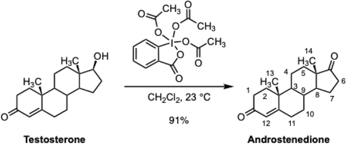
To a solution of testosterone (600 mg, 2.08 mmol, 1 equiv) in dichloromethane (105 ml, C = 0.020 M), Dess–Martin periodinane (3.53 g, 8.32 mmol, 4.00 equiv) was added. The reaction mixture was stirred for 2 h and diluted with water (150 ml). The diluted product mixture was transferred to a separatory funnel and the layers that formed were separated. The aqueous layer was further extracted with dichloromethane (2 ×50 ml), and the combined organic layers were dried over sodium sulfate. The dried solution was filtered and the filtrate was concentrated. The residue was purified by flash column chromatography (eluting with 10% ethyl acetate–hexane initially, then at a linear gradient to 30% ethyl acetate–hexane) to afford the androstenedione as a white solid (540 mg, 91%). Dess–Martin periodinane is potentially explosive and may be sensitive to heat and impact, particularly when impure. It should therefore be handled with appropriate precautions. Characterization data for androstenedione are as follows:
Rf = 0.49 (50% ethyl acetate–hexane; UV)
\({[{\rm{\alpha }}]}_{{\rm{D}}}^{20}\): +183 (c 0.55, CHCl3) 1H NMR (500 MHz, CDCl3) δ 5.74 (s, 1H, H12), 2.51–2.25 (m, 5H, 2 ⋅ H1, 2 ⋅ H11, 1 ⋅ H6), 2.16–2.06 (m, 1H, 1 ⋅ H2), 2.06–2.00 (m, 1H, 1 ⋅ H2), 1.99–1.93 (m, 2H, 1 ⋅ H7, 1 ⋅ H10), 1.89–1.81 (m, 1H, 1 ⋅ H5), 1.77–1.62 (m, 3H, 1 ⋅ H4, 1 ⋅ H6, H9), 1.55 (tt, J = 12.5, 9.1 Hz, 1H, 1 ⋅ H7), 1.44 (qd, J = 13.2, 4.2 Hz, 1H, 1 ⋅ H4), 1.34 – 1.22 (m, 2H, 1 ⋅ H5, H8), 1.19 (s, 3H, H13), 1.10 (qd, J = 12.9, 4.3 Hz, 1H, 1 ⋅ H10), 0.97 (ddd, J = 12.3, 10.7, 4.2 Hz, 1H, H3), 0.90 (s, 3H, H14).
13C NMR (126 MHz, CDCl3) δ 199.6 (C), 170.6 (C), 124.2 (CH), 53.9 (CH), 50.9 (CH), 47.6 (CH2), 38.7 (CH2), 35.8 (CH2), 35.8 (CH2), 35.2 (CH), 34.0 (CH2), 32.7 (CH2), 31.4 (CH2), 30.8 (CH2), 21.8 (CH2), 20.4 (CH2), 17.5 (CH3), 13.8 (CH3). One quaternary carbon was not observed. All NMR spectra are provided in Supplementary Figs. 1–4.
HRMS-CI (m/z): [M + H]+ calculated for C19H27O2 = 287.2006; observed peak = 287.2003.
Reporting summary
Further information on research design is available in the Nature Portfolio Reporting Summary linked to this article.