
Ethics
This research study did not require approval from any specific ethics board/committee.
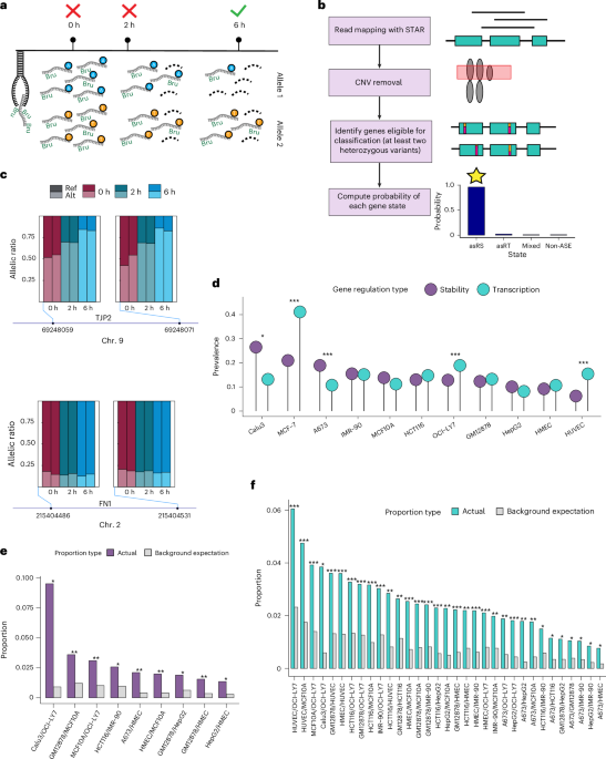
CNV removal
We obtained absolute copy numbers generated by the Cancer Cell Line Encyclopedia (CCLE)39 using the ABSOLUTE algorithm40. These copy number calls were overlapped with the GENCODE v.36 gene annotation. Only genes that overlapped copy number regions in which the minor ABSOLUTE copy number call and the major ABSOLUTE copy number call were equal to 1 were retained in downstream analysis.
If ABSOLUTE calls were not available, we used the CNVpytor41 software with bin size set to 10 kb to analyze cell lines that had publicly available whole-genome sequencing data (Supplementary Table 1 for data sources). We then filtered the CNV calls by requiring P value < 0.0001, CNV size ≥50,000 and at least half of the reads to be uniquely mapped. We used the default mean-shift caller for cell lines that are diploid or near diploid and the joint-caller for cell lines that are known to be polyploid (Supplementary Table 1).
For the remaining cell lines, we downloaded Hi-C data in pairs format (standard text format for pairs of genomic loci given at 1 bp point positions) and used ‘cload’ from the cooler42 software to convert these files into *.cool matrices at 20 kb resolution. We used the ‘calculate-cnv’ and ‘segment-cnv’ modules from NeoloopFinder43 to identify CNV regions in each cell line using the Hi-C cool files as input. ‘calculate-cnv’ was run with the ‘–enzyme’ parameter set to uniform and ‘segment-cnv’ was run with bin size 1,000 and ploidy set to two (default) for all cell lines except for Caco-2, in which ploidy was set to three. All genomic segments with copy number!= 2 were considered CNV regions. We filtered out genes if they overlapped any predicted CNV region.
Identification of asRS, asRT and mixed genes with RNAtracker
To categorize a gene as asRS, asRT or mixed, RNAtracker fits a beta-binomial mixture model (Supplementary Notes 2 and 3) for the reference allelic counts of the gene’s testable SNVs (total read counts ≥10 and minor read count ≥2) at each timepoint. Combining three timepoints (0 h, 2 h, 6 h), RNAtracker categorizes genes into one of seven possible states (listed in the table below), where each state is a triplet corresponding to three timepoints. At each timepoint, a gene is encoded as 1 for ASE and 0 for non-ASE. We denote the total count of the ith SNV of a gene g at timepoint t by \({{n}}_{{gi}}^{{t}}\), among which we assume the reference allelic count follows \({\text{beta-binomial}}({{n}}_{{gi}}^{{t}},{{\alpha}}_{0}^{{t}},{{\beta}}_{0}^{{t}},)\) if gene g is non-ASE or \({\text{beta-binomial}}({{n}}_{{gi}}^{{t}},{{\alpha}}_{1}^{{t}},{{\rm{\beta }}}_{1}^{{t}})\) if gene g is ASE, t = 0, 2, 6. Since we do not want to assume that the reference allelic count is always greater than the alternative allelic count, we ensure the beta distributions are symmetrical by setting the two beta distribution parameters equal, that is, \({{{\alpha}}_{0}^{{t}}={{\beta}}_{0}^{{t}},{\alpha}}_{1}^{{t}}={{\beta}}_{1}^{{t}}\). Specifically, in our implementation, we assume the reference allelic counts at 2 h and 6 h share the same parameters. To summarize, we have distributions at timepoints t = 0 following \({\text{beta-binomial}}({{n}}_{{gi}}^{0},{{\alpha}}_{0}^{0},{{\beta}}_{0}^{0},)\) if gene g is non-ASE or \({\text{beta-binomial}}({{n}}_{{gi}}^{0},{{\alpha}}_{1}^{1},{{\beta}}_{1}^{1})\) if gene g is ASE; at t = 2 or 6 following \({\text{beta-binomial}}({{n}}_{{gi}}^{{t}},{{\alpha}}_{0}^{2,6},{{\beta}}_{0}^{2,6})\) if gene g is non-ASE or \({\text{beta-binomial}}({{n}}_{{gi}}^{{t}},{{\alpha}}_{1}^{2,6},{{\beta}}_{1}^{2,6})\) if gene g is ASE.
0 h
2 h
6 h
State 0 (non-ASE)
0
0
0
State 1 (asRS)
0
1
1
State 2 (asRS)
0
0
1
State 3 (asRT)
1
1
1
State 4 (mixed)
1
0
1
State 5 (mixed)
1
0
0
State 6 (mixed)
1
1
0
First, in a preprocessing step, we focused on the 0 h data only and assumed that the reference allelic counts of each gene either follow the ASE beta-binomial distribution or the non-ASE beta-binomial distribution. Only genes with at least two testable SNVs are evaluated. We used \({{{\uppi }}}_{1}^{0}\) to represent the probability of a gene being ASE (or \({{{\uppi }}}_{0}^{0}=1-{{{\uppi }}}_{1}^{0}\) for a gene being non-ASE) at 0 h, where π refers to a fixed (nonrandom) parameter (or unknown constant) to be estimated. The expectation–maximization (EM) algorithm is then used to estimate the parameters \(({{\uppi }}_{1}^{0},{{\alpha}}_{0}^{0},{{\alpha}}_{1}^{0})\).
Upon convergence of the EM algorithm, we labeled each gene as non-ASE (0) or ASE (1) at 0 h based on the gene’s posterior probabilities for the two states. Our assignment of genes to the two states is a two-step procedure: first, we assigned every gene to the state at which its posterior probability is greater than 0.5; second, based on the initially assigned genes, we retained a gene in a state only if its posterior probability at that state is at least (1) 0.95 or (2) the first tercile of the posterior probabilities of all genes initially assigned to that state.
Second, after determining whether the gene exhibits ASE at 0 h in the preprocessing step, RNAtracker jointly considers data from the 2 h and 6 h timepoints to categorize genes into one of the seven triplet states. For genes that are labeled non-ASE in the previous step, the EM algorithm is used to estimate parameters \({{\alpha}}_{0}^{2,6},{{\alpha}}_{1}^{2,6},{{{\uppi }}}_{0}^{2,6},{{{\uppi }}}_{1}^{2,6}\), the first two of which are defined as the symmetric hyperparameters for the beta-binomial representing non-ASE and ASE genes, respectively, at each of the latter two timepoints (2 h and 6 h) and the last two of which are defined as the probability of a gene being in state 0 or state 1, respectively. The probability of a gene being in state 2 is \({{{\uppi }}}_{2}^{2,6}=1-{{{\uppi }}}_{0}^{2,6}-{{{\uppi }}}_{1}^{2,6}\). Similarly, for genes that are labeled ASE in the previous step, the EM algorithm is used to estimate parameters \({{\alpha}}_{0}^{2,6},{{\alpha}}_{1}^{2,6},{{{\uppi }}}_{3}^{2,6},{{{\uppi }}}_{4}^{2,6},{{{\uppi }}}_{5}^{2,6}\). Again, \({{\alpha}}_{0}^{2,6}\) and \({{\alpha}}_{1}^{2,6}\) are defined as the symmetric hyperparameters for the beta-binomial representing non-ASE and ASE genes respectively at each of the latter two timepoints (2 h and 6 h), and \({{{\uppi }}}_{3}^{2,6},{{{\uppi }}}_{4}^{2,6},{{{\uppi }}}_{5}^{2,6}\) are defined as the probability of a gene being in state 3, state 4 or state 5, respectively. The probability of a gene being in state 6 is \({{{\uppi }}}_{6}^{2,6}=1-{{{\uppi }}}_{3}^{2,6}-{{{\uppi }}}_{4}^{2,6}-{{{\uppi }}}_{5}^{2,6}\).
We then used a procedure similar to the two-step procedure utilized in the preprocessing step, with an additional refinement step to assign genes to the seven states. In step 1, we assigned every gene to the state with the highest posterior probability. In step 2, based on the initially assigned genes, we retained a gene in a state only if its posterior probability at that state is at least (1) 0.95 or (2) the first tercile of the posterior probabilities of all genes initially assigned to that state. Finally, in step 3, for each gene, we require at least half of its SNVs at each ASE timepoint (encoded as 1 in the table above) to exhibit allelic imbalance in the same direction across the two replicates. In other words, at least half of the SNVs in the gene must have the same sign (reference allelic ratio − 0.5) for the two replicates. Genes that fail this threshold are considered uncategorized.
To summarize, for the three timepoints, the RNAtracker model has a total of ten independent parameters \(\left(\!\right.{{\alpha}}_{0}^{0},{{\alpha}}_{1}^{0},{{\uppi}}_{1}^{0},\)\({{\alpha}}_{0}^{2,6},{{\alpha}}_{1}^{2,6},{{\uppi}}_{0}^{2,6},{{\uppi}}_{1}^{2,6},{{\uppi}}_{3}^{2,6},{{\uppi}}_{4}^{2,6},{{\uppi}}_{5}^{2,6}\left.\!\right)\) and three parameters that are constrained by \({{{\uppi }}}_{0}^{0}=1-{{{\uppi }}}_{1}^{0}\), \({{\uppi }}_{2}^{2,6}=1-({{\uppi}}_{0}^{2,6}+{{\uppi }}_{1}^{2,6})\) and \({{{\uppi }}}_{6}^{2,6}\)\(=1-({{\uppi}}_{3}^{2,6}+{{\uppi}}_{4}^{2,6}+{{\uppi}}_{5}^{2,6})\). Our justification for the model parameterization (in which parameters for 0 h are estimated separately from the 2 h and 6 h data) is that we want to implement stringent thresholds for calling genes ASE or non-ASE at 0 h, as this timepoint is crucial to distinguishing asRS from asRT genes. Moreover, the distribution of reference allelic counts at 0 h was found to be distinct from that of 2 h and 6 h; hence, the beta-binomial parameters are the same for 2 h and 6 h, but different from 0 h.
For details on the criteria for testable SNVs, identification of ASE SNVs, estimation of initial hyperparameters, and an extended explanation of RNAtracker, please refer to Supplementary Note 1.
Cell-type comparisons
To calculate the background expectation of shared asRS genes between each pair of cell lines, we obtained the number of asRS genes in each cell line and divided each value by the number of common testable asRS genes. The product of these two values was used as the background expectation, that is, the expected proportion of overlap. A binomial test was used to evaluate whether the background expectation differed from the actual proportion of shared asRS genes between the two cell lines. The same analysis was applied to asRT genes.
GTex analysis
Significant GTEx cis-eQTLs were downloaded from the GTex portal (v.8 release) at https://www.gtexportal.org/home/datasets (filename: GTEx_Analysis_v8_eQTL.tar). Fisher’s exact test was used to compute the odds ratio (that is, enrichment) of asRS or asRT variants overlapping significant GTEx cis-eQTLs compared to background variants. Background variants were those found in genes categorized as non-ASE by RNAtracker. For each overlap, we required the eQTL-associated gene to match the asRS, asRT or background gene. We also compared the enrichment of asRS and asRT genes among eGenes using Fisher’s exact test. This analysis was performed per tissue using asRS or asRT events combined across all cell lines (Fig. 2b), as well as in each cell line separately (Extended Data Fig. 7b).
Deep transcriptomic profiling of ActD-treated cells
RNA-seq (NovaSeq X Plus 150 PE) was performed for GM12878, MCF-7 and HCT116 cells before treatment with 10 μg ml−1 (GM12878, HCT116) or 5 μg ml−1 (MCF-7) of ActD, as well as 2 h, 8 h and 24 h post-treatment (three replicates per timepoint). These reads were processed using the same procedure as the Bru/BruChase-seq data (that is, STAR mapping with WASP filtering, followed by obtaining read counts at heterozygous SNV positions). To confirm the genotypes for these three cell lines, we sequenced their genomic DNA and called variants using the GATK germline short-variant discovery pipeline (https://gatk.broadinstitute.org/hc/en-us/articles/360035535932-Germline-short-variant-discovery-SNPs-Indels). To be considered validated, we required asRS genes to have at least one SNV that is non-ASE at 0 h but ASE at a latter timepoint. The allelic imbalance at the latter timepoint must be more extreme than the 0 h timepoint and at least 0.1 in at least one replicate. Alternatively, if the SNV is ASE at 0 h, its allelic imbalance must be more extreme at a latter timepoint and be at least 0.1 in at least one replicate. In either case, the direction of the allelic imbalance must be consistent with what is observed in the Bru/BruChase-seq data.
We used our previous approach in which we derive an empirical Gaussian distribution for the read coverage of each SNV to evaluate the probability that the average read count of the minor allele was generated from the same distribution as that of the major allele22. A SNV was deemed ASE if its Benjamini–Hochberg adjusted P value was less than 0.05. Allelic imbalance is calculated based on the delta allelic ratio at each SNV position: delta allelic ratio = abs(SNV allelic ratio − 0.5).
Prime editing
Prime editing was performed using the PE7 approach, which features a prime editor protein (PE7) fused to the RNA-binding, N-terminal domain of the small RNA-binding exonuclease protection factor La44. For each asRS variant that we evaluated with prime editing, we designed spacer and extension sequences for engineered prime editing guide RNAs (epegRNAs) using pegFinder45. pegLIT46 was used to design linker patterns for each epegRNA. Golden Gate assembly was used to clone the spacer, extension and epegRNA scaffold sequences (Supplementary Table 9) into the pU6-tevopreq1-GG-acceptor vector (Addgene, catalog number 174038) for epegRNA constructs. We then transfected pCMV-PE7 (Addgene, catalog number 214812) and the plasmid expressing each epegRNA into HEK293T cells, respectively. gDNA was extracted 72 h post-transfection to confirm genome editing events. Total RNA was then harvested from cells 0 h (pretreatment) and 2 h, 8 h and 24 h after treatment with 10 μg ml−1 of ActD (three replicates per timepoint). gDNA was also harvested from cells before ActD treatment (0 h). After reverse transcription using the SuperScript IV Reverse Transcriptase (Thermo Fisher Scientific, catalog number 18090010), the cDNA was amplified using gene-specific primers (Supplementary Table 9) to generate amplicons containing the variant of interest. Amplicons containing different variants from the same timepoint were pooled together before a second round of PCR to add Illumina adapters for sequencing. The PCR reactions were stopped before the plateau of the amplification curves. The libraries were purified using 2% agarose gel and sequenced with NovaSeq X Plus 150 PE.
Adapters were trimmed with bbduk (https://sourceforge.net/projects/bbmap/) before reads were mapped to GRCh38 with STAR (v.2.7.8a)47. To focus on reads from mature mRNA sequences, we filtered out unspliced reads before quantifying variant allelic counts with perbase (https://github.com/sstadick/perbase). Variants with a significantly different (Student’s t-test; P < 0.05) allelic ratio at post-ActD treatment timepoints (2 h, 8 h or 24 h) compared to the 0 h pretreatment timepoint were identified as causal variants.
Massively parallel reporter assays
A total of 365 asRS variants (Supplementary Table 5) were included in the MPRA experiment (following the MapUTR26 screening method) in HeLa cells. In brief, synthetic DNA oligonucleotides containing the variants of interest and their flanking sequences (164 nucleotides total) were cloned into the 3′ UTR of the eGFP gene. The expression of this reporter gene was driven by the cytomegalovirus early enhancer/chicken beta actin (CAG) promoter. These oligos were then introduced into HeLa cells by electroporation. Following electroporation (24 h), total RNA was extracted for sequencing targeting the tested variant regions. Specifically, the test sequences were amplified from both the plasmid library and mRNA to generate DNA sequencing and RNA-seq libraries. Three biological replicates were collected for each experiment and a high correlation was observed between replicates (R = 0.84). Sequencing data of the plasmid DNA and mRNA were compared to identify sites associated with significant expression differences between the two alleles using MPRAnalyze48. FDR ≤ 0.1 and |ln(FC)| ≥ 0.1 were required to call significance.
tamVars identified by MPRAu27 were obtained from Supplementary Table 1 of the corresponding study. Variants identified as a tamVar in at least one of the tested cell lines were considered functional variants.
Functional enrichment analysis
Allele-specific binding sites were obtained from our previous work (Supplementary Data 2 from ref. 22. After removing coordinate-unstable positions49, we converted ASB sites from hg19 to hg38 coordinates to be consistent with the asRS variants. eCLIP data for reproducible peaks (as determined from the irreproducible discovery rate approach50) were downloaded from the ENCODE portal. Annotations for RBP functions were obtained from Supplementary Data 1 from ref. 50.
rsids for SNPs overlapping miRNA seed regions that create or disrupt miRNA binding sites were downloaded from miRNASNPv3 (ref. 25). To be included in the enrichment analysis, these SNPs were required to be in the seed regions of miRNAs that were expressed in the cell line under consideration (nonzero read counts in miRNA-seq; Supplementary Table 1).
Each asRS variant was matched with a control variant that was sampled randomly from the same chromosome and type of genomic region (that is 3′ UTR, 5′ UTR, coding exon or exon in noncoding transcripts). asRS variants that appeared in more than one genomic context were assigned one control variant per genomic context. We overlapped all asRS and control variants with each set of functional annotations. For ASB and miRNA targeted sites, the proportion of asRS and control variants that overlapped each set of sites was calculated per cell line. Two-sided Wilcoxon’s signed-rank test was then used to assess whether the asRS variant proportion was significantly greater than the control variant proportion. For the eCLIP annotations, we used two-sided Fisher’s exact test to calculate enrichment of asRS variants that overlapped each set of functional annotations compared to control variants. The enrichment test was performed using the combined list of asRS and control variants across all cell lines. A pseudocount of 1 was added to avoid division by zero errors.
GO enrichment analysis
GO terms were downloaded from Ensembl using biomaRt51. The enrichment analysis was performed using all asRS genes as the set of query genes. For each asRS gene, a random control gene with gene length and average gene expression (across all samples) within 10% relative to that of the asRS gene was chosen. A total of 10,000 sets of control genes were obtained and a Gaussian distribution was fit to the number of control genes containing each GO term. This distribution was used to calculate the enrichment P value of the GO term among all asRS genes. Focusing on significant (FDR < 0.05) GO terms with at least five asRS (or asRT) genes, we then used rrvgo52 to group terms by semantic similarity (threshold = 0.7). rrvgo assigns parent terms to each group based on the GO term that has the most significant enrichment P value. Groups with two or more GO terms are shown in Fig. 4b. The ‘innate immune response’ cluster was renamed ‘immune response’ to more accurately describe the range of GO terms within this group.
GWAS catalog analysis
All reported associations were downloaded from the GWAS catalog (17 April 2023) and filtered to include variants that passed genome-wide significance at P < 5 × 10⁻⁸. We obtained GRCh38 genotype reference files from the 1000 Genomes project (subsampled for the EUR and CEU populations) (https://www.internationalgenome.org/data-portal/data-collection/grch38). Tag SNPs (required to be within 250 kb and exhibit r2 ≥ 0.8 with the target variant) were generated using plink (v.1.90)53 for all 2,242 asRS variants that were present in the genotype reference files. The overall enrichment of asRS variants that shared tag SNPs (across all traits) with significant GWAS associations compared to a random set of control variants was computed using two-sided Fisher’s exact test.
S-LDSC regression54 was used to estimate disease heritability. This analysis was run on all available harmonized summary statistics (31 January 2025) from GWAS catalog that were categorized under the EFO term EFO0000540 (immune system disease). Variant sets were defined by all genic variants inside asRS genes as determined by RNAtracker. LD scores for the regression were calculated using genotype reference files from 1000 Genomes project EUR samples within the variant sets for each chromosome. Disease heritability was then calculated using summary statistics for each disease of interest (Supplementary Table 7b), and s.e. values for heritability estimates were computed using the jackknifing approach. We required the enrichment s.e. to be less than the estimated enrichment for the result to be reported in Supplementary Table 7b.
Gene prediction of disease
Gene prediction models were built using the FUSION.compute_weights.R script from http://gusevlab.org/projects/fusion/. We matched each trait of interest to disease-relevant GTEx tissues (Supplementary Table 8). Subsequently, the genotypes and gene expression from each GTEx tissue of interest was used to compute gene prediction models for matched traits using variants that resided within asRS genes. The FUSION.assoc_test.R script was then used to estimate gene-disease associations.
Statistics and reproducibility
No statistical method was used to determine sample size. Sample size was set based on the number of Bru/BruChase-seq samples available through the ENCODE portal. We excluded data from cell lines that had an insufficient (<100) number of testable genes after CNV filtering. The experiments were not randomized. The investigators were not blinded to allocation during experiments and outcome assessment. Randomization and blinding were not relevant for our study given that samples were not allocated into experimental groups. The software (including specific version) and statistical tests used in the data analysis have been reported in Methods to facilitate reproducibility of the results.
Reporting summary
Further information on research design is available in the Nature Portfolio Reporting Summary linked to this article.