
Dataset and preprocessing
Our dataset includes PSG recordings from four different sites: SSC, BioSerenity, MESA20,21 and MROS20,22, with SHHS20,23 serving as an external validation dataset. Among these, MESA, MROS and SHHS are publicly available datasets, whereas SSC is our proprietary dataset. The BioSerenity dataset, provided by the BioSerenity company, contains 18,869 overnight recordings lasting 7–11 h each. This dataset is a subset of a larger collection from SleepMed and BioSerenity sleep laboratories, gathered between 2004 and 2019 across 240 US facilities19. At the time of this study, approximately 20,000 deidentified PSGs were available for analysis. The dataset distribution across different splits is shown in Fig. 1, with SSC constituting the largest cohort. To prevent data leakage, participants with several PSG recordings were assigned to a single split. For MESA, MROS and SHHS details, we refer readers to their original publications. Below, we describe our internal SSC dataset in more detail.
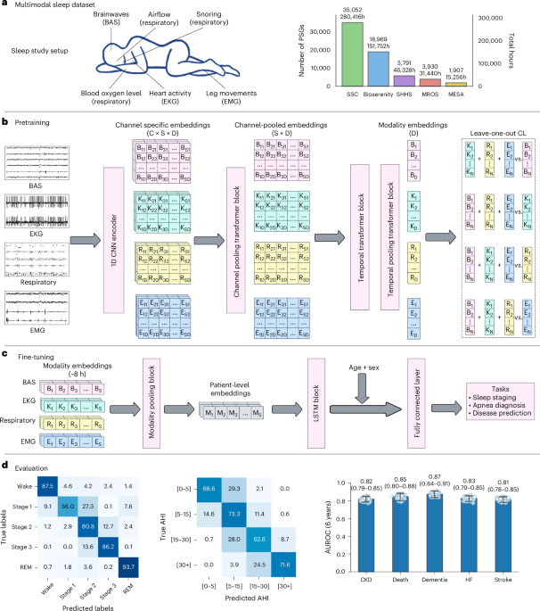
The SSC dataset comprises 35,052 recordings, each lasting approximately 8 h overnight. It includes diverse waveforms such as BAS, ECG, EMG and respiratory channels, making it a high-quality resource for sleep-related research. The dataset spans recordings from 1999 to 2024 and includes participants aged 2 to 96 years. The patient demographic statistics for SSC and BioSerenity are summarized in Extended Data Tables 1 and 2, respectively.
Our preprocessing strategy minimizes alterations to preserve raw signal characteristics crucial for identifying nuanced patterns. Each recording contains up to four modalities: BAS, ECG, EMG and respiratory, with variable numbers of channels. For BAS, we allowed up to ten channels, for ECG two channels, for EMG four channels and for respiratory seven channels. The number and type of channels vary across sites and even between patients within the same site, depending on the study type. The types of channel available across sites are described in Supplementary Tables 15–19. BAS includes channels that measure brain activity from different regions (frontal, central, occipital) as well as EOG for eye movements. EMG records electrical activity in muscles, whereas ECG captures cardiac electrical function. Respiratory channels measure chest and abdominal movements, pulse readings and nasal/oral airflow. These channels were selected based on their relevance to sleep studies, guided by sleep experts1.
Each PSG recording is resampled to 128 Hz to standardize sampling rates across participants and sites. Before downsampling, we utilized a fourth-order low-pass Butterworth filter to prevent aliasing, applied in a zero-phase setting to avoid phase distortion. Finally, we standardized the signal to have zero mean and unit variance. For any signals that needed to be upsampled, this was done using linear interpolation. Due to the channel-agnostic model design, we did not need any other data harmonization. Signals are segmented into 5-s patches, with each segment embedded into a vector representation for transformer model processing. To prevent data leakage, PSGs were split into pretrain, train, validation, test and temporal test sets early in the preprocessing pipeline. Although there is overlap between the pretraining and training sets, no overlap exists with the validation, test or temporal test sets. The SHHS serves as an independent dataset not used during pretraining, instead being used to evaluate the model’s ability to adapt to a new site through lightweight fine-tuning.
During pretraining, the only required labels are the modality types of the signals. A self-supervised CL objective is employed for pretraining. For downstream evaluations, we consider canonical tasks such as age/sex prediction, sleep stage classification, sleep apnea classification and various patient conditions extracted from EHR data. Sleep staging and apnea labels for SSC, MESA, MROS and SHHS were annotated by sleep experts. To ensure consistency across and within datasets, Rechtschaffen and Kales labels were converted to American Academy of Sleep Medicine standard by mapping Rechtschaffen and Kales stages 3 and 4 to American Academy of Sleep Medicine standard N3. SHHS also includes diagnostic information for conditions such as myocardial infarction, stroke, angina, congestive heart failure and death. For SSC, we paired PSG data with Stanford EHR data using deidentified patient IDs to extract demographic and diagnostic information. As BioSerenity lacks associated labels, it was used exclusively for pretraining.
SleepFM model architecture
Our model architecture is illustrated in Fig. 1. The architecture includes several key components that differ slightly between the pretraining and fine-tuning stages. During pretraining, we employ CL as the objective function for representation learning. A single model processes all four modalities.
The first component of the architecture is the Encoder, a 1D convolutional neural network (CNN) that processes raw signal data for each modality separately. The encoder takes raw input vectors, where the length of each vector corresponds to a 5-s segment of the signal, referred to as a token. The input dimensions are (B, T, C), where B is the batch size, T is the raw temporal length of the input and C is the number of channels for each modality. These inputs are reshaped into (B, C, S, L), where S is the sequence length representing the number of tokens (S = T/L) and L corresponds to the raw vector length for a single token (for example, 640 samples). Each token is then processed individually through a stack of six convolutional layers, each followed by normalization and ELU activation layers. These layers progressively reduce the temporal resolution while increasing the number of feature channels, converting the input from 1 channel to 128 channels. After this, adaptive average pooling further reduces the temporal dimensions, and a fully connected layer compresses the representation into a 128-dimensional embedding for each token. The final output of the encoder has dimensions (B, C, S, D), where D = 128.
Following the encoder, a sequence of transformer-based operations is applied to extract and aggregate modality-specific and temporal features. The first step is channel pooling, which aggregates token embeddings from all channels within a given modality. This operation uses an attention pooling mechanism based on a transformer layer to compute attention scores for each channel and produces a single aggregated embedding per time segment by averaging over the channel dimension. The resulting embeddings, with dimensions (B, S, D), are then passed through a temporal transformer, which operates along the temporal dimension to capture dependencies between tokens. The temporal transformer applies sinusoidal positional encoding to the token embeddings, followed by two transformer blocks consisting of self-attention and feedforward layers, enabling the model to learn contextual relationships across the sequence. After temporal modeling, the embeddings are processed through temporal pooling, which aggregates token embeddings over the sequence length (S) for each modality. Similar to channel pooling, temporal pooling uses an attention mechanism to compute weighted averages, generating a compact representation of size (B, 128) per modality. These steps collectively ensure that the model captures both spatial and temporal dependencies while reducing dimensionality for computational efficiency.
The final output is a single 128-dimensional embedding for each modality, used for CL during pretraining. Whereas the 5-min recordings are used exclusively for pretraining, we retain the 5-s-level embeddings for each modality for downstream tasks such as sleep staging and disease classification.
Baseline models
We evaluate SleepFM against two carefully chosen baseline approaches to demonstrate the value of our foundation model methodology.
The first baseline is a simple demographic model that processes only patient characteristics, including age, sex, BMI and race/ethnicity information. This demographic baseline is implemented as a one-layer MLP to establish a minimum performance threshold using only basic patient data available in most clinical settings.
The second baseline is the more sophisticated End-to-End PSG model that directly processes raw sleep recordings. This model uses the same architecture as SleepFM, including the 1D CNN encoder, channel pooling transformer block, temporal transformer block, temporal pooling transformer block and the LSTM layers, and is trained from scratch on the same dataset used for downstream evaluation. It also includes age and sex demographic features to ensure a fair comparison, but does not leverage any pretraining, serving to isolate the benefit of task-specific supervised learning on PSG signals without a foundation model.
All baseline models were trained using dataset splits shown in Table 1. The foundation model was first pretrained on the training dataset using a self-supervised objective, and subsequently fine-tuned on the same data. In contrast, the supervised baseline models were trained end-to-end without any pretraining. Although all models share identical architectures, training objectives and data splits, SleepFM consistently outperforms both baselines across a range of clinical prediction tasks. Although this may seem counterintuitive—given that the supervised PSG baseline is trained on the same data—these results align with well-established benefits of pretraining in representation learning. Self-supervised pretraining enables the model to learn more generalizable physiological representations, facilitates better convergence through improved initialization and makes more efficient use of sparse or noisy supervision during fine-tuning, as demonstrated in previous work11.
Model training
Model training can be categorized into two segments: pretraining and fine-tuning. The pretraining stage involves self-supervised representation learning with a CL objective and fine-tuning involves training the model with supervised learning objective for specific tasks such as sleep stage classification, sleep apnea classification and disease prediction. We describe these in more details below.
Pretraining
Model pretraining is performed using a self-supervised learning objective called CL. Specifically, we employ a CL objective for several modalities, referred to as LOO-CL. The key idea behind CL is to bring positive pairs of embeddings from different modalities closer in the latent space while pushing apart negative pairs. Positive pairs are derived from temporally aligned 5-min aggregated embeddings, obtained after temporal pooling, across four different modalities. All other nonmatching instances within a training batch are treated as negative pairs.
In LOO-CL, we define a predictive task where an embedding from one modality attempts to identify the corresponding embeddings from the remaining modalities. For each modality i, we construct an embedding \({\bar{x}}_{k}^{-i}\) by averaging over embeddings from all other modalities, excluding modality i. We then apply a contrastive loss between the embedding of modality i and this LOO representation:
$${{\mathcal{L}}}_{i,k}=-\log \frac{\exp \left({\rm{sim}}({x}_{k}^{i},{\bar{x}}_{k}^{-i})/\tau \right)}{\mathop{\sum }\nolimits_{m = 1}^{N}\exp \left({\rm{sim}}({x}_{k}^{i},{\bar{x}}_{m}^{-i})/\tau \right)},$$
where \({{\mathcal{L}}}_{i,k}\) is the loss for a sample k from modality i in a given batch, \({\rm{sim}}(\cdot )\) represents a similarity function (for example, cosine similarity) and τ is a temperature scaling parameter. The numerator computes the similarity between the embedding of modality i and the LOO representation of the corresponding sample, whereas the denominator sums the similarities across all samples within the batch. The motivation behind the LOO method is to encourage each embedding to align semantically with all other modalities.
Fine-tuning
After pretraining with the CL objective, we extract 5-s embeddings for all patient PSG data across modalities. We standardize the temporal context to 9 h for all patients—longer recordings are cropped and shorter ones are zero-padded to ensure consistent input dimensions. For example, for a patient’s standardized 9-h sleep data, the resulting patient matrix has dimensions (4 × 6,480 × 128), where 4 represents the number of modalities, 6,480 is the number of 5-s embeddings for 9 h of sleep and 128 is the embedding vector dimension.
During fine-tuning, we first apply a channel pooling operation across different modalities, reducing the dimensions to (6,480 × 128) for our example patient matrix. The pooled embeddings are then processed through a two-layer LSTM block, which is designed to handle temporal sequences. For sleep staging tasks, these 5-s embeddings are passed directly through a classification layer. For all other tasks, the embeddings are first pooled along the temporal dimension before being passed through an output layer.
For disease classification, we append age and sex features to the mean-pooled embedding vector after the LSTM block, before passing it to the final output layer. This addition empirically improves performance and surpasses the demographic baseline.
The fine-tuning objective for disease prediction uses the CoxPH loss function—a standard approach in survival analysis for modeling time-to-event data. The CoxPH loss maximizes the partial likelihood and is defined for a single label as:
$${{\mathcal{L}}}_{{\rm{CoxPH}}}=-\frac{1}{{N}_{e}}\mathop{\sum }\limits_{i=1}^{n}{\delta }_{i}\left({h}_{i}-\log \sum _{j\in R({t}_{i})}\exp ({h}_{j})\right),$$
where hi is the predicted hazard for the ith patient, δi is the event indicator (1 for event occurrence, 0 otherwise), ti is the event or censoring time, R(ti) represents the risk set of all patients with event times greater than or equal to ti, n is the total number of patients and \({N}_{e}=\mathop{\sum }\nolimits_{i = 1}^{n}{\delta }_{i}\) is the number of events.
For our multilabel setup with 1,041 labels, we extend the CoxPH loss by computing it independently for each label and summing the results:
$${{\mathcal{L}}}_{{\rm{total}}}=\mathop{\sum }\limits_{k=1}^{L}{{\mathcal{L}}}_{{\rm{CoxPH}}}^{(k)},$$
where L is the total number of labels.
Given the large dataset size, computing the loss for all patients in a single batch is computationally infeasible. Therefore, we calculate the loss in smaller batches of 32 samples, with patients sorted by event time in descending order to ensure correct computation of the partial likelihood. This batching strategy, combined with the summation of per-label losses, provides an efficient and scalable approach for multilabel time-to-event modeling.
Architectural details
We provide additional implementation-level details to clarify how SleepFM is constructed and trained. The design of SleepFM was developed through an empirical and iterative process, informed by domain knowledge and guided by practical training considerations. Although we did not perform an exhaustive hyperparameter search, we systematically evaluated architectural variants through trial-and-error by monitoring loss convergence, training stability and downstream performance.
Each 5-s segment of raw PSG signals (640 timepoints at 128 Hz) is passed through a tokenizer composed of six convolutional layers with increasing feature maps: 1 → 4 → 8 → 16 → 32 → 64 → 128. Each convolutional block includes BatchNorm, ELU activation and LayerNorm. After convolution, adaptive average pooling reduces the temporal axis to 1, and a linear layer projects the features to a fixed 128-dimensional token embedding. The resulting output shape is (B, C, S, 128), where C is the number of channels and S is the number of 5-s tokens.
To accommodate variability in the number and ordering of channels across different PSG datasets, we introduced an attention-based spatial pooling layer that operates across channels using a transformer encoder. This design makes the model robust to inconsistencies in recording configurations across sites. Specifically, embeddings from several channels within a modality are pooled using multihead self-attention, producing a modality-specific sequence of shape (B, S, 128).
To capture long-range temporal dependencies in sleep signals, the pooled token sequence is passed through three transformer encoder layers (each with eight heads, batch-first configuration and a dropout rate of 0.3), along with sinusoidal positional encoding and LayerNorm. This component enables modeling of contextual relationships across the sleep sequence. The output shape remains (B, S, 128).
An additional attention-based pooling layer aggregates the temporal sequence across timesteps, resulting in a single 128-dimensional embedding for each modality (for example, BAS, ECG, EMG or respiratory). These fixed-size modality-specific embeddings are used for pretraining with a self-supervised CL objective.
For downstream disease prediction, 5-s token embeddings spanning a standardized 9-h window are processed by a fine-tuning head. This head includes spatial pooling followed by a two-layer bidirectional LSTM (hidden size: 64). Temporal mean pooling is applied across valid timesteps, and normalized age and sex features are concatenated with the pooled output. The combined vector is then passed through a final linear layer to generate hazard scores for each disease. The total number of learnable parameters in this setup is approximately 0.91 million.
The supervised baseline model uses the same architecture as SleepFM but is trained from scratch without pretraining. The demographics-only baseline passes four input features—age, sex, BMI and race/ethnicity—through a shallow MLP with dimensions 4 → 128 → output.
Implementation details
All implementations were carried out using PyTorch, a library used widely for deep learning. The PSG data was gathered and processed within a HIPAA-compliant and secure compute cluster on Google Cloud Platform. Patient EHR data was likewise stored and analyzed exclusively within this secure environment.
For pretraining, the model was trained with a batch size of 32, a learning rate of 0.001, eight pooling heads, three transformer layers and a dropout rate of 0.3. As previously described, each patch size corresponds to a 5-s segment, and the total sequence length is 5 min for the transformer model. The total parameter count for the model was approximately 4.44 million. Pretraining was performed on 432,000 h of sleep data collected from 48,000 participants for one epoch, using an NVIDIA A100 GPU. The entire pretraining process took approximately 15 h.
For fine-tuning, the batch size was also set to 32, with a learning rate of 0.001, four pooling heads, two LSTM layers and a dropout rate of 0.3. The fine-tuned model had approximately 0.91 million learnable parameters. Training was conducted on patient data, with each token embedding represented as a 128-dimensional vector, over ten epochs. The fine-tuning process was performed on an NVIDIA A100 GPU, with the total training time per epoch ranging from 2 to 5 min, depending on the task.
All data analysis and preprocessing were performed using Python (v.3.10.14) and its data analysis libraries, including Pandas (v.2.1.1), NumPy (v.1.25.2), SciPy (v.1.11.3), scikit-survival (v.0.23.0), scikit-learn (v.1.5.2) and PyTorch (v.2.0.1).
Reporting summary
Further information on research design is available in the Nature Portfolio Reporting Summary linked to this article.