
All experiments complied with relevant ethical regulations. This study used established human cell lines and involved no human participants, human samples or animals; therefore, no human or animal ethics approval was required. Recombinant DNA experiments were approved by the Institutional Recombinant DNA Experiment Safety Committee of the National Institute of Genetics (R7-7). Additional experimental details are provided in Supplementary Methods.
Cell lines and culture conditions
HeLa S3 cells108 and HT1080 cells with lacO/EGFP-LacI and tetO/TetR-4×mCherry (a clone of TT75, TT165, kindly provided by T. Tanaka, University of Dundee)62 were cultured at 37 °C in 5% CO2 in DMEM (D5796-500ML, Sigma-Aldrich) supplemented with 10% FBS (FB-1061/500, Biosera). All HCT116 cells (CCL-247, ATCC) with AID2 for rapid depletion55 were cultured at 37 °C in 5% CO2 in McCoy’s 5 A medium (SH30200.01, HyClone) supplemented with 10% FBS.
Target protein depletion by AID2
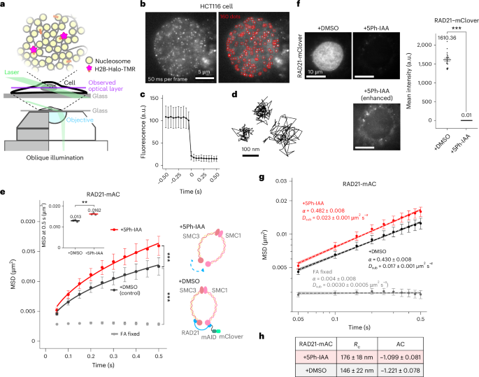
To rapidly degrade RAD21-mAC, CTCF-mAC and WAPL-mAC, HCT116 cells expressing OsTIR1(F74G) were treated with 1 µM 5Ph-IAA for 1 h (RAD21), 2 h (CTCF) or 4 h (WAPL), respectively, except where noted otherwise55,67. Control cells were treated with 0.1% dimethyl sulfoxide (D2650-5X5ML, Sigma-Aldrich). Degradation of the target proteins was confirmed by the loss of mClover fluorescence. After treatment, cells were fixed, permeabilized and stained with DAPI as described in the Supplementary Methods—‘Expression and localization of H2B-HaloTag or H3.3-HaloTag’. Z-stack images (30 sections at 0.2 µm intervals along the z axis) were acquired using a DeltaVision Ultra microscope (Applied Precision) equipped with an Olympus PlanApoN ×60 objective lens (NA 1.42). Nuclear mClover fluorescence intensity was quantified using Fiji, with background signal subtracted.
RAD21-mAC, WAPL-mAC or CTCF-mAC degradation was also confirmed by western blotting. The procedure was the same as described in the Supplementary Methods—‘Expression and localization of H2B-HaloTag or H3.3-HaloTag’. Membranes were probed with mouse anti-RAD21 (1:1,000; 05-908, Upstate), rabbit anti-WAPL (1:1,000; A301-779A-T), rabbit anti-CTCF (1:1,000; 10915-1-AP, PGI Proteintech) and mouse anti-mAID (1:1,000; M214-3, MBL) antibodies, followed by horseradish peroxidase-conjugated goat antimouse secondary antibody (1:5,000; 170-6516, Bio-Rad), or antirabbit IgG DyLight 800 (1:5,000; SA5-35571, Invitrogen). As a loading control, a goat anti-GAPDH antibody (1:2,500; 12004158, Bio-Rad; StarBright Blue700 conjugated) was used.
Single-nucleosome imaging
Established cell lines were cultured on poly-L-lysine-coated glass-based dishes (3970-035, Iwaki). H2B-Halo or H3.3-Halo incorporated into nucleosomes was fluorescently labeled with 80 pM HaloTag TMR ligand for 20 min at 37 °C in 5% CO2, washed thrice with 1× HBSS (H1387, Sigma-Aldrich) and then incubated in the following media overnight before single-nucleosome imaging. HeLa S3 cells were observed in DMEM (21063-029, Thermo Fisher Scientific), and HCT116 cells in McCoy’s 5 A (1-18F23-1, BioConcept). These media were phenol red (PR) free and supplemented with 10% FBS. To increase the number of tracked nucleosomes when applying the RL algorithm for motion classification, H2B-Halo was labeled with 50 nM PA-JF646 (provided by the Lavis Lab, Janelia Research Campus)75 overnight using the same labeling procedure.
A live-cell chamber (INU-TIZ-F1, Tokai Hit) and digital gas mixer (GM-8000, Tokai Hit) were used to maintain cell culture conditions (37 °C, 5% CO2 and humidity) during microscopy. Single nucleosomes were observed using an inverted Nikon Eclipse Ti microscope equipped with a 100-mW Sapphire 561-nm laser (Coherent) and an sCMOS ORCA-Flash 4.0 or ORCA-Fusion BT camera (Hamamatsu Photonics). Live cells labeled with TMR were excited with the 561-nm laser through an objective lens (×100 PlanApo TIRF, NA 1.49; Nikon) and detected at 575–710 nm. An oblique illumination system with a TIRF unit (Nikon) was used to excite fluorescent nucleosome molecules within a thin area of the cell nucleus and reduce background noise (Fig. 1a). Sequential image frames were acquired using NIS-Elements (Nikon) at a frame rate of 50 ms under continuous illumination. Please note that freely diffusing, non-nucleosomal histones cannot be tracked at this frame rate. For PA-JF646-labeled nucleosome tracking, the cells were continuously photoactivated with weak 405-nm illumination (1.0 mW, 25% AOTF attenuation) together with 640-nm laser excitation.
To visualize the basal nuclear surface (nuclear periphery), we adjusted the angle of laser illumination to efficiently capture a nuclear membrane marker, NUP107-Venus109. Almost uniform distributions of NUP107-Venus were observed in the nuclear periphery condition, while the nuclear interior condition showed a rim of NUP107-Venus76. As reported previously76,77, nucleosome dynamics on the nuclear surface were lower than those of the nuclear interior, which contained more euchromatin regions. Position-determination accuracy is 7.3 nm (Extended Data Fig. 7g).
Single-nucleosome tracking analysis
To study nucleosome motion within chromatin domains accurately, we mainly focused on the 0–0.5 s time window, which corresponds to the spatial range of typical chromatin domain sizes (up to ~300 nm). At longer time scales, other factors, such as higher-order structures (for example, compartments, territories) and nuclear movements, become more influential (for details, see refs. 45,110). To obtain the Rc value57, we also analyzed longer-time data, up to ~3 s.
Image processing, single-nucleosome tracking and single-nucleosome movement analysis were performed as previously described5,41,45,76. Briefly, sequential images were converted to 16-bit grayscale, and background noise was subtracted using the rolling-ball background subtraction (radius, 50 pixels) in ImageJ. Nuclear regions in the images were manually extracted. The fluorescence dots were fitted with a 2D Gaussian function80,111 and tracked using u-track software112, or their centers were determined by LoG detector in Fiji plugin TrackMate113.
To assess positional accuracy, we calculated the s.d. of the 2D movement of immobilized nucleosomes per 50 ms in FA-fixed cells (n = 10 nucleosomes). We found that 12.5 nm (the mean of SDx and SDy) was the localization accuracy (Extended Data Fig. 1d). Single-step photobleaching profile confirmed that the individual dots represent single nucleosomes (Fig. 1c).
For single-nucleosome imaging/tracking, we calculated displacement and MSD of nucleosomes, because MSD captures the relevant constrained nucleosome dynamics, for the following reasons: the vast majority of the labeled histones are incorporated into nucleosomes constrained along a very long polymer rather than freely diffusing, and state mixing is minimal. In this respect, single-nucleosome imaging is very different from single-molecule tracking of transcription factors. MSD in single-molecule tracking of transcription factors can be error prone because multiple diffusion states (free 3D diffusion, one-dimensional sliding, specific binding) interconvert, and displacement-based analyses are often preferable (for example, ref. 114).
For single-nucleosome movement analysis, the displacement and MSD of the fluorescence dots were calculated based on their trajectory using a Python script. In our tracking, trajectories of single-nucleosome dots on the XY plane \({\left({{x}}_{i}\right)}_{i=0}^{n}\) were acquired, where xi indicates XY coordinates at the time point i. Then, we calculated the MSD for the lag time ∆ by:
$${\mathrm{MSD}}\left({\mathrm{lag}}\,{\mathrm{time}}\right)=\frac{1}{n-\Delta}\sum _{i=1}^{n-\Delta}{\left|{x}_{i}-{x}_{i+\Delta}\right|}^{2}$$
(1)
The originally calculated MSD was in 2D. To obtain the 3D value, the 2D value was multiplied by 1.5 (4 to 6 D × t). The calculated MSDs were fitted to a subdiffusive model MSD(t) = 6D × ta, where α is an anomalous diffusion exponent (0 < α < 1). Statistical analyses of the obtained single-nucleosome MSD captured through each histone protein were performed using Python.
The anomalous exponents (α) and the coefficient of subdiffusion Dsub were obtained from the slope and the intercept of the log–log MSD plots by linear regression within the 0–0.5 s time window, respectively. Graphs and statistical analyses of single-nucleosome MSD under different conditions were performed using R. For Spot-on analysis114, single-nucleosome trajectory data taken with 10 ms per frame were analyzed. The three-state model is used for model fitting.
Sample preparation for SIM imaging
Two days before labeling, cells were grown on poly-L-lysine-coated, super-resolution-grade coverslips (No. 1S; 0.17-mm thickness; CS01803, Matsunami). H3.3-Halo in HCT116 cells was fluorescently labeled by incubating the cells for more than 1 h with 50 nM TMR. Cell fixation and immunostaining were performed as described in the Supplementary Methods—‘Verification of DNA damage’. Fixed cells were observed at room temperature.
To experimentally ‘melt’ the euchromatin domains, the cells were treated with TSA (203-17561, Wako) for 7 h before fixation. For the double treatment with TSA and acute cohesin depletion, cells were also treated with 1 µM 5Ph-IAA for the final 1 h. Histone hyperacetylation and RAD21 depletion were confirmed by western blotting. The western blotting procedure was described in the Supplementary Methods—‘Expression and localization of H2B-HaloTag or H3.3-HaloTag’. Membranes were probed with rabbit anti-acetyl H3 (1:2,000; 06-599, Millipore), rabbit anti-acetyl H4 (1:2,000; 06-866, Millipore) and mouse anti-RAD21 (1:1,000; 05-908, Upstate) followed by horseradish peroxidase-conjugated goat antirabbit secondary antibody (1:5,000; 170-6515, Bio-Rad) or antimouse IgG secondary antibody (1:5,000; 170-6516, Bio-Rad). As a loading control, a mouse antilamin A/C antibody (1:1,000; sc-7292, Santa Cruz) was used.
For live imaging, cells were grown on poly-L-lysine-coated glass-based dishes. H3.3-Halo incorporated into nucleosomes was fluorescently labeled with 50 nM HaloTag TMR ligand for 1 h at 37 °C in 5% CO2, washed thrice with 1× HBSS and then observed in PR-free McCoy’s 5 A at 37 °C in 5% CO2.
For immunostaining, cells were incubated with diluted primary antibodies in 1% NGS in HMK for 1 h—mouse anti-RAD21 (1:1,000; 05-908, Upstate), mouse anti-RNAP II CTD (1:1,000; ab817, Abcam), mouse anti-RNAP II Ser5P (1:1,000; provided by Hiroshi Kimura, Science Tokyo) or mouse anti-RNAP II Ser2P (1:1,000; provided by Hiroshi Kimura, Science Tokyo) antibody. After four washes with HMK, cells were incubated with diluted secondary antibodies in 1% NGS in HMK for 1 h—goat antimouse IgG Alexa Fluor 488 (1:500; A11029, Invitrogen) or goat antimouse IgG Alexa Fluor 647 (1:500; A21236, Invitrogen), followed by four additional washes with HMK. DNA staining and mounting were performed as described in the Supplementary Methods—‘Expression and localization of H2B-HaloTag or H3.3-HaloTag’.
3D-SIM microscopy
SIM was performed on a Nikon N-SIM S system (Ti-2 stand; Hamamatsu ORCA-Fusion BT camera; Nikon Perfect Focus; Chroma ET525/50 m, ET595/50 m and ET700/75 m emission filters). A Nikon ×100 PlanApo TIRF oil-immersion objective (NA 1.49) was used. NIS-Elements (Nikon) software was used to control the system and acquire 3D-SIM images. Illumination was provided by ZIVA light engines (Lumencor) containing 405, 476, 545 and 637 nm lasers. Light was directed to the sample through a specific filter for each channel.
Here 3D image stacks were acquired over the entire cell volume in z, with 15 raw images per plane (five phases and three angles). Optical sectioning images were acquired at 0.12 µm intervals, with a total of 51 sections covering the entire nucleus (6 µm in thickness). Images acquired on the Nikon N-SIM-S system were reconstructed and corrected for chromatic aberrations using stack reconstruction in the NIS-Elements software.
System performance and both raw and reconstructed data quality were carefully assessed and optimized using the SIMcheck ImageJ plugin (Extended Data Fig. 8a–e)79. To exclude potential false-positive nuclear marker signals, we applied the modulation contrast-to-noise ratio (MCNR) map function of SIMcheck, which generates a metric of local stripe contrast across different regions of the raw data and directly correlates this with the level of high-frequency information content in the reconstructed data79. Only immunofluorescence spot signals with MCNR values above a stringent quality threshold were considered, whereas localizations with low MCNR values were discarded as unreliable SIM signals.
Classification analysis for 3D-SIM images
The 3D assessment of DAPI intensity classes or H3.3-Halo intensity classes as a proxy for chromatin compaction was performed as previously described107,115. First, 1,000 was subtracted from all voxel intensity values to remove background noise, and nuclei were cropped. Nuclear voxels were automatically identified from the DAPI channel using Gaussian filtering and thresholding through the ‘dapimask’ function in the ‘nucim’ R package.
For chromatin quantification, a 3D nuclear mask was generated to define the region for segmenting DAPI or H3.3-Halo signals into seven intensity classes with equal variance, following the method discussed in refs. 7,107. In brief, voxel-wise classification was performed using a hidden Markov random field model that combines a finite Gaussian mixture model with a spatial Potts model, implemented in R. This approach enables threshold-independent classification of chromatin compaction states at the voxel level based on the DAPI or H3.3-Halo intensity. Heatmaps of the seven intensity classes in individual nuclei were generated using Fiji and displayed in either color or grayscale. The relative volume of each class was calculated as the volume of that class divided by the total nuclear volume detected by DAPI staining.
Power-spectrum analysis for 3D-SIM images
Single midsections from individual nuclei were cropped from the original reconstructed 3D-SIM images. The cropped images were then converted to 2D Fourier spectra using Python116. The resulting power spectra were radially averaged to analyze the amplitude at specific spatial periodicities.
STORM imaging
HCT116 RAD21-mAC H3.3-Halo cells were cultured on poly-L-lysine-coated glass-based dishes (3970-035, Iwaki). H3.3-Halo incorporated into nucleosomes was labeled with 100 nM HMSiR-Halo (A201-01, Goryo Chemical) in medium for 3 h at 37 °C in 5% CO2. Cells were washed thrice with PR-free McCoy’s 5A medium (PR-free McCoy’s 5A) with 10% FBS and then incubated with PR-free McCoy’s 5A with 10% FBS and 0.1% dimethyl sulfoxide or 10% FBS and 1 µM 5Ph-IAA for 1 h. Cells were fixed with 3.7% FA (064-00406, Wako) in Opti-MEM (31985062, Gibco) at 37 °C in 5% CO2 for 15 min, washed thrice with PR-free McCoy’s 5A with 10% FBS and observed in PR-free McCoy’s 5A with 10% FBS.
Single molecules were observed using an inverted Nikon Eclipse Ti-2 microscope with an ILE laser unit (ANDOR) and the sCMOS ORCA-Fusion BT camera. Fluorescent molecules in living cells were excited by the 640-nm laser through an objective lens (×100 Apo TIRF, NA 1.49; Nikon) and detected. An oblique illumination system with a TIRF unit (TI2-LA-TIRF-E, Nikon) was used to excite labeled molecules within a limited thin area in the cell nucleus and reduce the background noise. Sequential 5,000 images were acquired using NIS-Elements (Nikon solutions) at a frame rate of 10 ms under continuous illumination. To maintain cell culture conditions (37 °C, 5% CO2 and humidity) under the microscope, a live-cell chamber with a digital gas mixer and a warming box (Tokai Hit) was used.
STORM images were constructed using the Fiji package ThunderSTORM117 based on sequential images of HMSiR. For clustering analysis, TrackMate was also used for localization. The estimated localization accuracy is 4.546 nm for x and 4.672 nm for y (Extended Data Fig. 8f).
To estimate the individual cluster size, we used the SR-Tesseler-DBSCAN pipeline82. First, SR-Tesseler is used with a low-density factor (0.7) to extract chromatin regions, then DBSCAN (with 90-nm distance and 100 minimum samples) detects each cluster.
Dual-color labeling and imaging
HCT116 RAD21-mAC H3.3-Halo cells were cultured on poly-L-lysine-coated glass-based dishes (3970-035, Iwaki). H3.3-Halo incorporated into nucleosomes was sequentially labeled, first with 200 nM PA-JF549 (ref. 75) for 20 min and then with 50 nM PA-JF646 (ref. 75) for 20 min at 37 °C in 5% CO2. Cells were washed thrice with 1× HBSS (H1387, Sigma-Aldrich) and incubated in PR-free McCoy’s 5A medium for more than 1 h before single-nucleosome imaging (Extended Data Fig. 9h,i).
Simultaneous dual-color imaging in live HCT116 cells was performed under the same conditions as described in ‘Single-nucleosome imaging’, except that a beam splitter (W-VIEW GEMINI, Hamamatsu Photonics) was used, equipped with an image-splitting dichroic beam splitter (FF640-FDi01-25 × 36, Hamamatsu Photonics) and bandpass filters (FF01-593/40-25 and FF01-676/29-25, Hamamatsu Photonics). The cells were continuously photoactivated with weak 405-nm illumination (1.0 mW, 25% AOTF attenuation).
Two-point MSD analysis
In our single-nucleosome tracking, trajectories of PA-JF549-labeled and PA-JF646-labeled nucleosomes on the XY plane, \({\left\{{{\mathbf{{S}}}}_{549}\left({t}_{m}\right)\right\}}_{m=0}^{M-1}\) and \({\left({{\mathbf{{S}}}}_{646}\left({t}_{m}\right)\right)}_{m=0}^{M-1}\), were simultaneously acquired, with a time interval of Δt = 0.05 s and tm = mΔt(m = 0, 1, 2,…, M − 1). To evaluate dynamic fluctuations between two points, we considered the relative vector between two trajectories, Q ™ = S549 ™ − S646 ™. Then, we calculated the two-point MSD for the lag time tn = nΔt by
$$\text{MSD}\left({t}_{n}\right)={\left\langle \frac{1}{M-n}\mathop{\sum }\limits_{m=0}^{M-1-n}{\left[{\mathbf{{Q}}}\left({t}_{m+n}\right)-{\mathbf{{Q}}}\left({t}_{m}\right)\right]}^{2}\right\rangle }_{{t}_{n}}\times \frac{3}{2}$$
where \({\left\langle \cdot \right\rangle }_{{t}_{n}}\) represents the ensemble average for trajectories at the lag time tn and the coefficient 3/2 is a correction factor for conversion from 2D to 3D values.
Statistics and reproducibility
No statistical method was used to predetermine sample size. Sample sizes were based on previous studies using the same imaging and analysis methods5,30,45. For cell-based experiments, a biological replicate was defined as an independently performed experiment using a separately prepared cell culture. The numbers of biological replicates and cells analyzed in each replicate, the definition of n, the statistical tests used and exact P values are provided in the figure legends of Figs. 1–8 and Extended Data Figs. 1–10 and in Supplementary Table 1. For the primary analyses of cell-to-cell heterogeneity (Figs. 1–4 and 7 and Extended Data Figs. 1, 3, 4, 7 and 9), measurements from individual cells pooled across biological replicates were used to compare distributions between conditions using the statistical tests indicated in the figure legends. In parallel, replicate-aware analyses were performed by summarizing individual-cell measurements within each biological replicate and using the resulting biological replicate-level values for statistical testing. These analyses were used to confirm that the differences observed in the pooled cell populations were reproducible across independent experiments. Paired tests were used when control and treatment conditions were measured in parallel within the same biological replicate. Where multiple pairwise comparisons were performed, P values were adjusted using the Holm method. All statistical tests were two sided unless otherwise stated. For parametric tests, data were assumed to follow a normal distribution, but this assumption was not formally tested. Data not meeting the technical or quality-control criteria described in the Methods subsections ‘Target protein depletion by AID2’, ‘Single-nucleosome tracking analysis’, ‘3D-SIM microscopy’ and ‘STORM imaging’, or in the Supplementary Methods subsections ‘Head-tethering of the cohesin’, ‘ATAC-seq experiments and data processing’, ‘Intron-seqFISH probe selection and design’ and ‘Intron-seqFISH’, were excluded from the analyses; no other data were excluded. The experiments were not randomized. The investigators were not blinded to allocation during experiments and outcome assessment. The numbers of independent repeats for experiments showing representative images are stated in the corresponding figure legends and Supplementary Table 1.
Reporting summary
Further information on research design is available in the Nature Portfolio Reporting Summary linked to this article.