
Study population
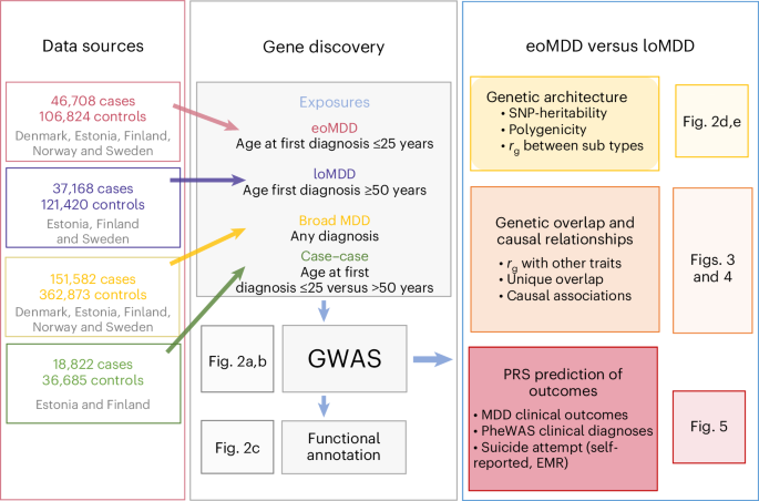
To conduct a large GWAS of AAO-based MDD subtypes with consistent phenotypes, we identified nine cohorts across five Nordic countries (Denmark, Sweden, Norway, Finland and Estonia), and a comparison cohort from a non-Nordic country (the UK: UKB). Many of these cohorts are large biobanks linked with lifetime medical records in national patient registers, including iPSYCH, FinnGen, the Norwegian Mother, Father and Child Cohort Study (MoBa), the UKB and the EstBB (cohort details in Supplementary Methods). This study was approved by the Swedish ethical review authority (case no. 2023-03073), and each cohort was approved by the relevant institutional review boards.
Phenotypes
We expanded our previous effort of harmonizing the register-based phenotypes of MDD, age at first diagnosis and its outcomes in the three Scandinavian countries to other Nordic countries with similar registers15. Using national patient registers, we first extracted information on patient diagnoses of MDD using ICD-10 code F32 (depressive episode) or F33 (recurrent depressive episodes), with the exclusion criteria of a lifetime diagnosis of bipolar disorder or schizophrenia (ICD-10 codes: F30/F31/F32/F33, F20/F23.1/F23.2/F25) (Supplementary Table 14), resulting in a total combined number of MDD cases in the Nordic countries of n = 151,582. Our previous research revealed a high genetic correlation (rg ≈ 0.95) between AAO and age at first diagnosis for MDD16, and that onset on average predates first diagnosis by 5 years16. Therefore, we derived the age at first diagnosis for the MDD patient population and used that as a proxy for AAO for the definition of eoMDD and loMDD. The cutoffs were chosen based on careful review of the literature and the empirical registry data from Sweden. Previous meta-analysis reported that the median AAO for depressive disorder is around age 30, with the 25th and 75th percentile at age 21 and 44, respectively15,19; our Swedish registry data showed that for age at first MDD specialist diagnosis, the 25th and 75th percentile were at age 25 and 45, respectively15. Thus, we considered individuals with their first psychiatric specialist treatment contact for MDD at or before age 25 (approximate to the 25th percentile of the AAO distribution at age 20–21) as cases with eoMDD (n = 46,708); cases with loMDD were those with their first specialist treatment contact for MDD at or after age 50 (approximate to the 25th percentile of the AAO distribution at age 44–45; n = 37,168). Controls were individuals without a registered diagnosis of MDD, bipolar disorder or schizophrenia. Because of the differences in cohort design, controls were matched to cases for the population-based cohorts of EstBB, FinnGen, MoBa and UKB. The Danish and Swedish cohorts, which used case–cohort and case–control designs, did not require control matching.
Software containers for federated analyses
To ensure transparent and reproducible analyses of data across sites, we developed software containers and accompanying codes for data processing and analyses (for example, GWAS, PRS, LDSC) and distributed the containers across the study sites. Briefly, the primary software tools and dependencies were installed in virtual machines based on the Ubuntu 20.04 LTS Linux operating system via Docker (https://docker.com) and containerized using the Singularity Image File format (https://sylabs.io) for distribution20. All source codes and files are publicly available via GitHub and released under the GNU General Public License (GPL v.3.0). Tools released under other licenses retain their original licenses.
GWAS and meta-analysis
GWAS of individuals with European ancestries was conducted in each cohort using the REGENIE software package37 available in the software containers20. Analyses were adjusted for the first ten principal components (PCs), age and sex. Summary statistics from each cohort were included in a fixed-effects meta-analysis in METAL38 with the ‘SCHEME STDERR’ command using the inverse variance weight of the corresponding standard errors for all phenotypes studied, resulting in 151,582 cases and 362,873 controls for all MDD, 46,708 cases and 106,824 controls for eoMDD, and 37,168 cases and 121,420 controls for loMDD. Additional variant filtering was applied: INFO score > 0.8, minor allele frequency ≥ 1% and n > 10,000. After this filtering, the numbers of markers for the final METAL analyses were 8,910,578 for broad MDD, 8,848,589 for eoMDD and 8,820,060 for loMDD. Genome-wide significance was set at P < 5 × 10⁻⁸. Genome-wide loci were identified based on genome-wide significant SNPs using PLINK (–clump command). A gene list was then created based on which genes physically overlapped the loci from the previous step (Supplementary Table 2). An additional case–case GWAS was performed comparing eoMDD cases to loMDD cases using the EstBB and FinnGen cohorts, as they include both eoMDD and loMDD cases in their biobanks. A total of 32,060 samples from FinnGen and 23,447 samples from EstBB were meta-analyzed using METAL; heritability \(\left({h}_{{\rm{SNP}}}^{2}\right)\) was estimated using LDSC39,40.
Gene-based tests
We used MAGMA41 v.1.08 to test the aggregate association of variants by assigning SNPs to genes. Gene boundaries were expanded by 35 kb upstream and 10 kb downstream to allow for the inclusions of promoters and cis-enhancers. We used the updated deep whole-genome sequencing of the 1000 Genomes Project (European subset) as reference data42, downloaded from http://ftp.1000genomes.ebi.ac.uk/vol1/ftp/data_collections/1000G_2504_high_coverage/working/20220422_3202_phased_SNV_INDEL_SV/.
Tissue-type and cell-type enrichment of SNP heritability with stratified LDSC
We used stratified LDSC39 to perform tissue-type and cell-type analysis, estimating the enrichment of SNP heritability in a set of genome annotations. We downloaded precomputed LDSC scores from https://console.cloud.google.com/storage/browser/_details/broad-alkesgroup-public-requester-pays/LDSCORE/LDSC_SEG_ldscores/biorxiv/Roadmap_1000Gv3.tgz, containing data on 396 annotations of epigenetic marks from the ROADMAP project, restricting to the 102 annotations relating to the brain. For the gene expression data, we followed our previous protocol43, first aggregating gene expression across genes to get the average expression per gene in each cell type. We then defined cell-type specificity by dividing the expression of a gene in a cell type by its total expression across all cell types. For each cell type, we considered the top decile of specifically expressed genes as typifying that cell type, and computed LDSC scores for that annotation. In addition to the ROADMAP annotations, we also tested the enrichment of SNP-based heritability (one-sided) in human tissues (37 human tissues from GTEx28) and brain cell types using the latest human single-nucleus transcriptomic data (31 major human brain cell types from ref. 29). We applied a Bonferroni correction for multiple testing in each annotation and trait (for example, in the analysis of ROADMAP data, significance was set at P < 0.05/102 for each trait).
SNP-based heritability and assessing genetic overlap
We used LDSC to estimate SNP-based heritability and genetic correlation40. To convert the SNP-based heritability to the liability scale, we calculated the sample prevalence of cases in the meta-analysis; for population prevalence, we used a lifetime estimate of diagnosed MDD of 16% (ref. 44). To obtain corresponding estimates for eoMDD and loMDD, we estimated the proportion of cases with MDD who had an early-onset or a late-onset diagnosis in the largest population samples (EstBB and FinnGen) and took that as a percentage of the whole MDD prevalence estimate, resulting in a population estimate of 6.2% for eoMDD and 3.2% for loMDD. Acknowledging that these estimates are approximations, we provided SNP heritability estimates for a range of prevalence estimates (±50% around the point estimates).
To estimate genetic correlations with other traits, we used phenotypes from publicly available summary statistics, selecting important psychiatric disorders and key health determinants and outcomes, including suicide, body mass index, educational attainment, substance use, mortality and cardiovascular disease (GWAS sources in Supplementary Table 15).
SBayesS
Using SBayesS30, we confirmed the LDSC estimates of SNP-based heritability and further estimated the parameter of polygenicity, that is, the proportion of SNPs with nonzero effects, and negative selection. We used the precomputed LD Matrix from UKB participants (‘ukbEURu_imp_v3_HM3_n50k.chisq10’), which is available from the software authors. We ran four chains in parallel to estimate the convergence across starting parameters (–num-chains 4), with each run consisting of 25,000 iterations (–chain-length 25,000), with 5,000 iterations considered as burn-in iterations (–burn-in 5,000).
Genomic SEM
We used genomic SEM to compare the extent to which genetic liability to eoMDD versus loMDD overlaps with genetic liability to other phenotypes45. Genomic SEM is an extension of SEM whereby GWAS summary statistics are used to capture the ‘observed’ traits in the model so that the genetic architecture underlying the multivariate relationships between traits can be modeled. Genomic SEM relies on LDSC to estimate genetic correlations and is robust to any amount of sample overlap. We modeled the association of the MDD subtypes with other related phenotypes that have been well studied in the literature, including a range of psychiatric disorders, important health determinants, CVD and mortality (Supplementary Table 15). First, we compared the size and significance of the genetic correlations of the two subtypes (eoMDD and loMDD) with the other phenotypes. Next, we assessed the subtype-specific contribution to the other phenotypes by controlling for the other subtype (for example, we investigated the relationship between eoMDD and suicide attempt after controlling for loMDD). Thus, the unique contribution of each can be gauged while controlling for their shared variance. The genetic overlap between eoMDD and loMDD was moderate; therefore, the concern for strong bias through multicollinearity was limited.
Mendelian randomization
Following the analyses of genetic overlap, we used MR to assess whether the MDD subtypes were causally associated with selected health outcomes (risk factors, mortality and CVD; Supplementary Table 15). We did not include psychiatric outcomes because of the high likelihood of pleiotropy. Assuming that alleles are randomly distributed in the population (in a manner akin to experimental randomization), MR uses genetic variants as instrumental variables to capture a trait (‘exposure’). If the genetic variants are robust, non-pleiotropic instruments for the exposure and there is no direct association with the outcome or an unmeasured confounder, this provides support for a potential causal effect of the exposure. We conducted main and sensitivity analyses as implemented in the TwoSampleMR R package46 and computed the IVW statistic to estimate these associations. For interpretation, we focused on effect consistency across tests, rather than P values. Still, to give an indication of the extent of the multiple testing burden, we report significance according to false discovery rate-corrected P values (Benjamini–Hochberg method). We present several sensitivity analyses that correct for potential violations of the MR assumptions. Weighted median and mode analyses are more robust to invalid instruments and correct for outliers47. The MR-Egger analysis was used to assess any remaining pleiotropy (intercept) and adjust for such effects. The MR-Egger estimate is often underpowered, but it is still informative to check whether the effect is in the same direction as the other sensitivity analyses48. From the same TwoSampleMR package, it is possible to estimate the amount of heterogeneity (Q) in the SNP effects, and estimate the instrument strength F. We added a sensitivity analysis from the MR-PRESSO R package49, which has a different and more powerful way to adjust for the effects of outliers and is aimed at correcting for pleiotropy. Finally, we assessed the ‘no measurement error’ assumption by deriving the I2 statistic and applied a SIMEX correction on the MR-Egger estimate if I2 was between 0.6 and 0.8 (we did not present the MR-Egger estimate when the I2 fell below the 0.6 cutoff50). Although we were not able to remove potential sample overlap from the analyses (LOO analyses would leave the exposure GWAS underpowered), this should not be a large threat to the validity of our results. The extent of bias stemming from sample overlap is limited if the sample size of the source GWAS is large, the overlap is small and the heritability of the investigated traits is high51. As shown in Supplementary Table 15, the amount of sample overlap was limited in most cases and present only for a subset of traits.
The aim of the MR analyses was to contrast causal associations between eoMDD and loMDD. However, there was overlap in the instrument sets for both traits. Although only one SNP is present in both sets, many had LD partners in common. Therefore, we performed another sensitivity analysis using a single instrument SNP for each trait. We selected the genome-wide significant SNP that had the largest P value for the other trait (filtering on a minor allele frequency > 0.10). For eoMDD, we used rs7622302 residing in the DAG1 gene on chromosome 3, with P = 0.98 for loMDD. This instrument explained 2.8% of the variance (R2) in eoMDD. For loMDD, we used rs3777421 in the IGF2R gene on chromosome 6, with P = 0.87 for eoMDD. This SNP explained 2.7% variance in loMDD. Although power was expected to be lower in these single-SNP analyses, pleiotropy was also reduced; instrument strength was still sufficient (F = 30.7 for eoMDD and F = 30.1 for loMDD) and the contrast between eoMDD and loMDD was maximized.
Polygenic risk scores
PRS were calculated using LDpred252, which addresses some limitations of LDpred53. Briefly, LDpred2 is a Bayesian method that uses the LD structure in the genome combined with priors regarding the genetic architecture of a trait (SNP heritability and fraction of causal SNPs (hyperparameter p)) to compute PRS. We used the ‘auto’ method of LDpred2 that maximizes the predictive performance of the PRS by testing a range of the fraction of causal SNPs. For our analyses, we used LD matrices provided by the authors of LDpred252, which were generated from the UKB samples (European ancestry) with 1.1 million HapMap3 SNPs. The LDpred2 calculations relied on the bigsnpr R library54 and were implemented in a set of custom R scripts55.
Individual-level PRS in each cohort were computed using the LOO GWAS summary statistics on MDD subtypes and tested for associations with clinical characteristics or MDD-related outcomes (Supplementary Table 16) in logistic regression models adjusted for at least ten PCs (cohort-dependent), sex and birth year. For the outcomes that were available in all target samples, we performed fixed-effects meta-analysis using the R package metafor56.
PRS PheWAS
To investigate the genetic comorbidity of eoMDD and loMDD, we conducted a PRS PheWAS using logistic regression models, using the EstBB electronic health record (EHR) data. Analyses were performed in R (v.4.3). For each ICD-10 code with at least 50 cases (n = 1,151) present in the EstBB EHR, two models were constructed—eoMDD PRS and loMDD PRS as the predictor. These models used the normalized PRS (either eoMDD or loMDD) and a binary outcome variable indicating the presence or absence of the ICD-10 code. The EHR data encompassed both primary and secondary/inpatient care data through linkage to the Estonian central e-health database, covering the time from 2004 to 2022.
The models included sex, year of birth and the first ten genetic PCs as covariates. To account for multiple testing, we applied Bonferroni correction, resulting in a conservative P threshold of 0.05/1,151. ORs (with 95% CIs), the number of cases per ICD-10 code and the P values for both eoMDD and loMDD models are provided in Supplementary Table 12 and Supplementary Figure 8a,b.
Self-reported suicidality stratified according to eoMDD PRS
To evaluate the effect of the eoMDD PRS on self-reported suicidality, we used data from the EstBB Mental Health Online Survey57. Self-reported suicidality was assessed using the Paykel Suicide Scale, which includes five items assessing self-reported suicidal thoughts and attempts32. A total of 58,732 individuals who had an MDD diagnosis were present in the EHRs (F32 or F33 codes) and responded to the Paykel Suicide Scale. For this analysis, the first four questions were scored on a scale from 0 to 4 (0 indicating the participant had never felt or experienced this, and 4 indicating the participant felt or experienced it often). The fifth question had binary responses (no/yes) corresponding to values of 0 or 2. The total score of the five items was used for the analysis; the distribution according to eoMDD PRS group is provided in Supplementary Table 13a. The mean values and standard deviations of these sums were then computed for three groups based on eoMDD PRS deciles (1st, 2nd to 9th, 10th). Analyses were conducted using R (v.4.3).
Cox proportional-hazards model of suicide attempt stratified according to eoMDD PRS
To estimate the absolute risk of EHR-based suicide attempt over 10 years after the first diagnosis of MDD, stratified according to eoMDD PRS, we used a Cox proportional-hazards model58, using data from the EstBB (results in Supplementary Table 13). Sex and year of birth were included as covariates. The analysis included a cohort of 10,539 individuals diagnosed with MDD (first diagnosis date in 2000 or later, identified by the ICD-10 codes F32 or F33, before or at the age of 25). Participants’ birth years ranged from 1974 to 2004, with a mean birth year of 1990.
We calculated the absolute risk (with 95% CIs) of suicide attempt after the first episode of depression for three groups based on eoMDD polygenic risk score deciles: the 1st decile, the 2nd to 9th deciles and the 10th decile. The risk of suicide attempt was assessed over a 10-year period (3,650 days) after the initial MDD diagnosis. ICD-10 codes X60-X84 and Y87 from the Estonian EHRs were used to identify suicide attempts. The absolute risk was presented as 1 minus the survival probability. All analyses were conducted using R v.4.3, with the ggsurvfit (v.1.0.0)58 and survival (v.3.5.7) packages59.
Reporting summary
Further information on research design is available in the Nature Portfolio Reporting Summary linked to this article.