Paired mutation calling and spatial transcriptomics identify cellular neighborhoods associated with the neoplastic outcome of mouse colitis

Mice

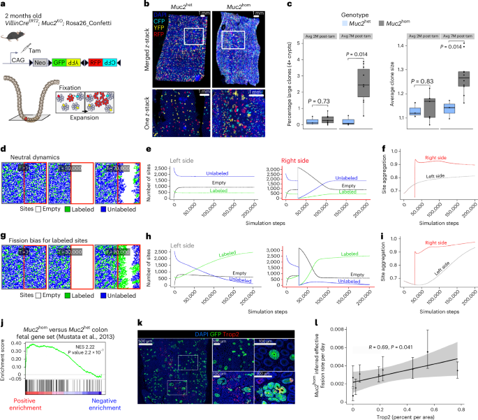
Mice were of C57BL/6 background. The Muc2KO line used was described by Velcich et al.16. Mice containing inter-crossed R26Confetti and VillinCreERt2 alleles18 were bred to Muc2KO mice to generate VillinCreERt2; Muc2KO; R26Confetti mice. To model sporadic colon carcinogenesis, the intestinal epithelium-specific inducible Cre VillinCreERt2 line was crossed with Apcfl/+(ref. 58). All genotyping was outsourced to Transnetyx.

Animal husbandry

Animal care and procedures were performed at the Cancer Research UK Cambridge Institute Biological Resource Unit according to the UK Home Office under the authority of a Home Office project licence (PD5F099BE) approved by the Animal Welfare and Ethical Review Body at the CRUK Cambridge Institute, University of Cambridge. Mice were housed under controlled conditions (temperature (21 ± 2 °C), humidity (55% ± 10%), 12 h light–dark cycle) in a specific-pathogen-free facility (tested according to the recommendations for health monitoring by the Federation of European Laboratory Animal Science Associations). Animals had unrestricted access to food and water. None of the mice had been involved in any procedure before the study. To trigger acute inflammation, 2% DSS was provided in drinking water for 5 days. To trigger colon carcinogenesis, 200 mg kg−1 ENU was injected intraperitoneally. Mice which showed clinical signs of tumor burden (anemia, hunching and loss of body condition) before experimental endpoints were culled and removed from the study.

Human tissue

Colon tissue samples were obtained from patients with IBD and/or CAC at St James University Hospital Leeds under full local research ethical committee approval (12/LO/1217 approved by London–Bloomsbury Research Ethics Committee) according to the Health Research Authority institution. Patient consent was obtained at the time of surgery, and they did not receive compensation. Colectomy specimens were fixed in 10% neutral buffered formalin and embedded en face in paraffin (FFPE) blocks.

Three-dimensional imaging and clone counting

The whole colon of VillinCreERt2; Muc2KO; R26Confetti mice was dissected, flushed with cold PBS, cut longitudinally and whole-mounted. Following fixation in 4% paraformaldehyde overnight at 4 °C, the tissue was washed in PBS and selected colon segments were excised. Optical clearing was performed using the CUBIC protocol59. In brief, excised segments were incubated with CUBIC-1a solution (10% urea, 5% N,N,N′,N′-tetrakis(2-hydroxypropyl) ethyl-enediamine, 10% Triton X-100 and 25 mM NaCl in distilled water) at 37 °C for 7–10 days with alternate day solution changes. 4′,6-diamidino-2-phenylindole (DAPI) was used for nuclear counterstaining at a dilution of 1:1,000. The cleared tissue was then washed in PBS for 24 h. Additional clearing and refractive index matching were performed with Rapiclear 1.52 (152002, SunJin Labs) for 24 h. Samples were mounted in a 0.25-mm i-Spacer (Sunjin Labs) for confocal imaging on a Leica SP5 TCS confocal microscope (LAS software v2.8.0, Leica Biosystems) with a 10× objective, 1.4–1.7 optical zoom and 8–12 μm z-steps throughout the whole thickness of the tissue. Clone counting was performed using the cell counter tool in the ImageJ software.

Immunohistochemistry

Mouse colons were opened longitudinally and cut in approximately 15-mm2 sections placed in cassettes and fixed overnight at 4 °C in 4% paraformaldehyde. H&E staining was performed using an automated ST5020 Multistainer (Leica Biosystems). Staining for β-catenin was performed on Leica’s automated Bond-III platform in conjunction with the Polymer Refine Detection System (DS9800, Leica Biosystems). In brief, epitope retrieval was performed using Leica Epitope Retrieval Solution 1 (AR9961, Leica Biosystems) at 100 °C. Blocking was performed with Protein Block Buffer (X090930-2, Dako). Following incubation with primary antibody against β-catenin (0.25 μg ml−1, mouse, 610154, BD Biosciences), sections were incubated with secondary antibody (1:1,500, rabbit anti-mouse IgG1, ab125913, Abcam) before development and mounting. For β-catenin staining, an additional mouse-on-mouse blocking step was performed.

Immunofluorescence

Heat-mediated epitope retrieval was performed on rehydrated 3-μm-thick paraffin sections in 10 mM sodium citrate (pH 6.0). The sections were then incubated in blocking solution (10% donkey serum and 0.05% Tween-20 in PBS) at room temperature for 30 min. Primary antibodies against RFP (1:100, rabbit, R10367, Thermo Fisher), GFP (1:100, chicken, ab13970, Abcam), E-cadherin (1:200, mouse, 610182, BD Biosciences), Trop2 (1:100, goat, AF1122, R&D systems) and Arid1a (1:100, rabbit, 12354S, Cell Signaling) were diluted in blocking solution, in which sections were then incubated in the dark overnight at 4 °C. Sections were washed and incubated with fluorophore-conjugated secondary antibodies (donkey anti-rabbit A31572, donkey anti-goat A21447 and/or donkey anti-chicken 703-6-5-155, Thermo Fisher and/or donkey anti-mouse ab150109, Abcam) diluted 1:200 in 0.05% Tween-20 in PBS for 45 min at room temperature. DAPI (1:1,000) was used for nuclear counterstaining. After washing, the stained sections were mounted using ProLong Gold Antifade Mountant (P36930, Thermo Fisher).

RNAscope

Simultaneous detection of Notum and Reg4 was performed on paraffin embedded sections using Advanced Cell Diagnostics (ACD) RNAscope 2.5 LS Duplex Reagent Kit (322440), RNAscope 2.5 LS Probe- Mm- Notum C1 (428988) and RNAscope 2.5 LS Probe-Mm-Reg4-C2 (409608). The 3-µm-thick sections were baked for 1 h at 60 °C before loading onto a Bond RX instrument (Leica Biosystems). Slides were deparaffinized and rehydrated on board before pre-treatments using Epitope Retrieval Solution 2 (AR9640, Leica Biosystems) at 95 °C for 15 min and ACD Enzyme from the Duplex Reagent kit at 40 °C for 15 min. Probe hybridization and signal amplification were performed according to manufacturer’s instructions. Fast red detection of C2 was performed on the Bond Rx using the Bond Polymer Refine Red Detection Kit (DS9390, Leica Biosystems) according to ACD protocol. Slides were then removed from the Bond Rx and detection of the C1 signal was performed using the RNAscope 2.5 LS Green Accessory Pack (322550, ACD) according to kit instructions. Slides were heated at 60 °C for 1 h, dipped in xylene and mounted using VectaMount Permanent Mounting Medium (H-5000, Vector Laboratories). The slides were imaged on the Aperio AT2 (Leica Biosystems) to create whole slide images. Images were captured at 40× magnification, with a resolution of 0.25 μm per pixel.

Inference of effective fission rate from lineage tracing data

The statistical model for crypt fission described in Nicholson et al.22 and implemented in the R package RHClones (https://github.com/ElEd2/RHClones) was adapted to infer effective fission rates using counts of clone sizes from n = 3 equal size tissue areas from n = 3 Muc2het and n = 3 Muc2hom mice with different average Trop2 expression levels, selected at random. Clone sizes were counted manually using the ImageJ cell counter tool, then the number of pixels stained with Trop2 was obtained using the Area tool in the measure function in ImageJ. Each tissue region was assigned a local fission rate \({\rho }_{i}\) (units, per day) that is sampled from a hierarchical Student’s T prior

$${\rho }_{i}\, \sim \,{StudentT}\left(\nu ,\mu ,\sigma \right)$$

with population-level parameters

$$\sigma \,\approx \,\mathrm{normal}\left(0,{10}^{-2}\right)$$

$$\sigma \,\approx \,\mathrm{normal}\,\left(0,{10}^{-2}\right)$$

$$\nu \,\approx \,\mathrm{gamma}\left(2,{10}^{-1}\right).$$

The vector of observed clone sizes, \({{\boldsymbol{g}}}_{i}\), for region i is then distributed according to

$${{\boldsymbol{g}}}_{i}\, \sim \,{Multinomial}\left({\boldsymbol{f}}({\rho }_{i},{t}_{i})\right)$$

where

$${{\bf{f}}}_{n}\left(\rho ,t\right)={{\rm{e}}}^{-\rho t}{(1-{{\rm{e}}}^{-\rho t})}^{n-1}$$

is the solution of the Yule–Furry pure birth process, and \({t}_{i}\) is the time (in days) since clone induction in region i.

The model for fission inference in this study differs from the model for fission after continuous clone induction described in Nicholson et al.22, where this solution is integrated over the age of the individual. However, as in the aforementioned study, a correction was applied to \({f}_{1}\) and \({f}_{2}\) to correct for the chance occurrence of neighboring, nonclonally related crypts. This model does not incorporate crypt fusion, nor does it account for tissue remodeling that may partly explain clone sizes in tissue areas associated with repair following inflammation. In this respect, inferred fission rates should be interpreted as ‘effective’ in the sense that they only capture the value of \({\rho }_{i}\) that is required to explain clone sizes using the Yule–Furry pure birth process introduced in Nicholson et al.22.

Simulations of crypt dynamics

Crypt dynamics were simulated using an on-lattice, voter-type model. The square lattice is of shape \(M\times M\). For a site \((i,{j})\) on the lattice, the neighboring sites are defined to be the set

$${N}_{i,j}\,=\left\{\left(i,\,j\,+\,1\right),\,\left(i,j-\,1\right),\,\left(i\,+\,1,\,j\right),\,\left(i-1,j\right),\,\left(i\,+\,1,\,j\,+\,1\right),\,\left(i\,-\,1,\,j-1\right)\right\}$$

resembling a configuration equivalent to a hexagonal lattice in two dimensions with periodic boundary conditions. The state of a lattice site \((i,{j})\), denoted by \({s}_{i,j}\), is defined as \({s}_{i,j}=-1\) for unlabeled (UL) sites, \({s}_{i,j}=0\) for empty sites and \({s}_{i,j}=+1\) for labeled (L) sites. Assuming a labeling efficiency of 20%, the initial population on the lattice consists of 80% of UL and 20% of L sites randomly assigned to each site. The parameters governing the simulations are the fission (\({\rho }_{s}\)), fusion (\({f}_{s}\)) and fixation (\({P}_{s}\)) probabilities of the state \(s=\pm 1\). All are assumed to be neutral and equal for L and UL crypts as the baseline scenario (\({\rho }_{s}\), \({f}_{s},\,{{P}}_{s}=\,0.5\) for \(s=\,\pm 1\), undefined otherwise). To determine the impact of fission bias in tissue repair, the fission probability of L sites was increased to \({\rho }_{1}=0.95\), with all other parameters remaining the same.

The simulation rules are that, at each time step, we choose a random site \(\left(i,{j}\right)\) and update the lattice state according to

1.

If \(\left(i,\,j\right)\) is an empty site \(\left({s}_{i,j}=\,0\right):\)

i.

All neighbors are empty sites \(({s}_{k,l}\,=\,0\,\forall \,\left(k,{l}\right)\in \,{N}_{i,j}\,),\) do nothing;

ii.

Otherwise, choose a nonempty neighbor site \(\left(k,{l}\right)\in {N}_{i,{j}}:\,{s}_{k,{l}}\ne 0\) at random to undergo fission by setting \({s}_{i,{j}}={s}_{k,l}\) with probability \({\rho }_{{s}_{k,l}}\) (Fig. 1a and Supplementary Fig. 1).

2.

If \((i,{j})\) is nonempty\(\,{(s}_{i,j}\ne 0)\), then choose a neighbor \(\left(k,{l}\right)\in {N}_{i,{j}}\) at random:

i.

If \(\left(k,{l}\right)\) is empty, then \((i,{j})\) undergoes fission by setting \({s}_{k,l}={s}_{i,j}\) with probability \({\rho }_{{s}_{i,j}}\);

ii.

Otherwise, fusion occurs with probability \(\frac{{f}_{{s}_{i,j}}+{f}_{{s}_{k,l}}}{2}\) by choosing \(\left(h,{w}\right)\in \{\left(i,j\right),(k,l)\}\) with equal probability and setting \({s}_{h,w}=0\). The outcome of monoclonal fixation following fusion is then determined to be the state \(s{\prime}\) according to the fixation probabilities \({P}_{{s}_{i,j}}\) and \({P}_{{s}_{k,l}}\) as outlined in Fig. 1b,c and Supplementary Fig. 1 and then setting \({s}_{p,q}=s{\prime}\) where \(\left(p,{q}\right)\in \{\left(i,j\right),\left(k,l\right)\}\backslash \{\left(h,{w}\right)\}\).

We note that our definition of homeostasis in in silico models is not equivalent to an equilibrium since, while the average numbers of labeled and unlabeled crypts remain constant, their spatial distribution across the lattice undergoes domain coarsening as captured by a ‘site aggregation’ metric that slowly increases across the course of simulations (Fig. 1f,l). Furthermore, fission-biased conditions lead to a nonhomeostatic system even in the absence of damage, as higher expansion rates generally outpace the creation of empty space by crypt fusion. This is reminiscent of a regime where additional mechanisms, such as diffusion (not considered here), may be required to spatially accommodate mutant crypts with higher rates of fission (Olpe et al.21).

Calculation of site aggregation

The number of distinct neighbor pairs (DNPs) was quantified to represent aggregation of labeled and unlabeled sites in the lattice. The number of the DNPs for a \((i,{j})\) on the lattice is defined to be the cardinality of the set

$${G}_{i,j}=\left\{\left({s}_{i,j}\,,\,{s}_{k,l}\right):\left(k,\,l\right)\in \,{N}_{i,j}\,,\,{s}_{i,j}\,\ne \,{s}_{k,l},\,{s}_{i,j}\,\ne 0,\,{s}_{k,l}\ne 0\right\}.$$

The neighbor pairs of a site (i, j) is the set:

$${K}_{i,j}=\left\{\left({s}_{i,j}\,,\,{s}_{k,l}\right):\left(k,\,l\right)\in \,{N}_{i,j}\,,\,{s}_{i,j}\,\ne 0,\,{s}_{k,l}\ne 0\right\}.$$

To obtain a measure of DNPs independent of grid size, we consider the concentration of DNPs, defined as

$$C=\,\frac{\alpha }{\beta }$$

where \(\alpha\) and \(\beta\) are the total number of DNPs and neighbor pairs over the whole lattice, respectively. Importantly, we considered aggregation of labeled and unlabeled sites, excluding empty sites and plotted site aggregation as \(1-C\), so that increasing values denote a decreasing concentration of DNPs.

Bulk RNA sequencing

RNA was collected from n = 3 Muc2hom and n = 3 Muc2het mouse colons from 10-month-old littermates. mRNA extraction was performed following instructions from the extraction kit (180244, Qiagen). Library prep was performed by the CRUK Cambridge Institute Genomics Core using the Illumina Stranded mRNA Prep kit (20040532, Illumina) according to manufacturer’s instructions. Samples were sequenced using the Illumina Novaseq platform with 50-bp paired end reads. Differential expression analysis was performed using DESeq2. Expressed genes were ranked by descending log2 fold change for use in gene set enrichment analysis60.

Setup for paired spatial transcriptomic and DNA sequencing

A cohort of five Muc2hom mice were treated with ENU 8 weeks post birth and aged for 16 more weeks before collection. Whole-mounted colons were fixed, and six serial tissue sections of 3–5-μm thickness were cut at the crypt base, for at least three areas per colon representing varied levels of pathology. Levels were used for: (1) spatial transcriptomics profiling, (2) pathology assessment with H&E, (3) tumor counting with β-catenin immunohistochemistry, (4) clone counting with GFP, RFP + DAPI and E-cadherin counterstain, and (5) Arid1a-mutated clone counting with Arid1a + DAPI counterstain.

Spatial transcriptomics

Slide processing and library preparation were performed according to the 10x Visium Cytassist FFPE protocol. In brief, 5-μm sections of tissue were transferred to fit each of the two 11-m2 oligo-barcoded capture areas on Visium 10x Genomics slides. Libraries were processed by the CRUK Cambridge Institute Genomics Core according to the manufacturer’s instructions and sequenced on Illumina’s NovaSeqX Plus to an average depth of 8 million mapped reads per sample. Fastq files were processed using the Spaceranger command line tool (10x Genomics v3.0.1) and mapped to the pre-built mm10 reference genome. Processed gene expression matrices for each slide were converted to a Seurat object. Number of counts and features were capped at a minimum of 500 and 200, respectively, to remove low quality spots. After normalization by variance stabilizing transformation using SCTransform, objects corresponding to each slide were integrated into a merged Seurat object using Harmony61. Clusters were identified using FindNeighbors using integration anchors at a UMAP dimension of 0.5. Genes differentially expressed in each cluster compared with all other clusters were derived using FindMarkers. To select top markers for each cluster, differentially expressed (DE) genes were filtered for expression in at least 50% of barcoded spots in one cluster (pct.1 >0.5) and expression in less than 50% of other clusters (pct.2 <0.3). This filtered list was ranked on descending log2 fold change and ascending P value and the top two markers per cluster were selected. For pseudo-bulk analysis, LoupeBrowser was used to extract barcoded spots assigned to each of the 2-mm-diameter biopsies from which DNA was sequenced.

Transfer of cluster labels

Cluster identities from a reference sample (SITSA1) were transferred to query samples (Muc2het and Muc2hom) using Seurat’s label transfer workflow. Reference and query objects were merged, SCT-normalized and PCA and UMAP dimensionality reduction were performed. The merged object was split by sample, and for each query, transfer anchors were computed on shared features using FindTransferAnchors. Cluster labels from the reference were then predicted with TransferData and added to each query as metadata. Query samples were saved by cohorts for downstream analysis.

DWLS cell-type deconvolution

Cell-type proportions in each barcoded spot were estimated using DWLS38. Cell-type signatures were derived from a single-cell RNA-sequencing dataset of ten mouse colons in different health conditions: n = 3 healthy, n = 3 acute DSS colitis and n = 4 chronic DSS colitis39 (accession GSE264408), using the author curated ‘major’ cell-type annotations with the top ten markers for each cell type. The average proportion of each cell type in each cluster was calculated by taking the mean of the DWLS-estimated fractions across all spots assigned to that cluster. Of note, the cellular origin of the tumor cluster 10 could not be appropriately defined using this healthy cell-type reference.

GSVA

Variation in pathway activity between clusters was quantified using GSVA. Mouse Hallmark gene sets were obtained from MSigDB, excluding sets with fewer than five genes. SCT-normalized expression data was used, after removing genes with near-zero variance (expressed in ≤1 spot). Pathway scores were scaled before downstream analyses. Differential pathway activity for each cluster was identified by comparing that cluster against all other clusters, using FindAllMarkers without thresholds for log fold change or minimum expression.

Correlation in cluster coverage

Correlations between proportions of barcoded spots mapping to the tumor cluster and other clusters were calculated based on symmetric balances for compositional parts data, as described by Kynclova, Hron and Filzmoser41. For each tumor and nontumor cluster pair, two sets of orthonormal coordinate systems were constructed according to symmetric balances of log ratios of either cluster relative to all other clusters in each sample. Pearson correlation coefficients for the first coordinate in each of the two coordinate systems then captures the association of nontumor cluster with the tumor cluster across samples: a positive correlation coefficient implies that enrichment of the two clusters over the respective ‘average representatives’ of other clusters increase simultaneously and vice versa for negative correlation. A coefficient of zero implies that enrichment of these two clusters is controlled by uncorrelated processes.

Pseudo-spatiotemporal mapping

SpaceFlow42 was used to combine expression matrices and spatial coordinates from spatial transcriptomics data in a graph-convolutional deep model, to produce low-dimensional embeddings reflecting both gene expression similarity and spatial proximity between barcoded spots. Pseudo-spatiotemporal maps (pSM) are a pseudotime-like ordering of the clusters according to the embeddings, as described in the original SpaceFlow paper.

Cluster correlation and matching for additional tumorigenesis models

Gene expression was correlated between clusters identified in the Muc2hom + ENU dataset, and the dataset integrating the Muc2hom + ENU cohort, as well as DSS + ENU, Apc + ENU, Muc2hom and Muc2het cohorts. For each dataset, average expression profiles were computed using Seurat (v5) and restricted to the set of DE genes detected in both datasets. DE genes (P value <0.05) were identified using Seurat’s FindAllMarkers function. To ensure comparability, the number of DE genes used per cluster was limited to 124, the smallest number of DE genes observed in any cluster in the reference dataset.

Pairwise Spearman correlation coefficients were computed between all ‘old’ (Muc2hom + ENU) and ‘new’ (full dataset) cluster mean expression vectors. For each old cluster, new clusters exhibiting a correlation coefficient <0.8 were identified as matched. Cluster correspondences were visualized using an alluvial plot generated with the ggalluvial R package (v0.12.5).

NGS library preparation with targeted DNA sequencing library assays

Genes of interest were imported in the Fluidigm D3 Assay design platform and dual coverage primers were designed (Supplementary Table 7). Eight amplicon pools were prepared and used in the LP 8.8.6 integrated fluidic circuit (101-7663) according to manufacturer’s instructions. Samples were sequenced in two separate runs by the CRUK Cambridge Institute Genomics Core on Illumina NovaSeqX Plus for 150-bp paired end reads.

Mutation calling

RePlow62 was used for mutation calling based on dual replicate amplicon coverage using combinatorial pooling of amplicons and applied to the first 20 million reads of each sample (Supplementary Table 7). In brief, RePlow exploits replicate library preparations to separate the contribution of background errors occurring in library preparation from sequencing errors occurring in sequencing. This is done with a statistical model that calculates the total log ratio of probabilities for variant candidates compared with background errors across all replicates simultaneously. In doing so, adjusted VAFs are constructed by subtracting the contribution from sequencing errors, whereas background error profiles for the error model are calculated independently for the six base pair substitution types (A > C, A > G, A > T, C > A, C > G, C > T) across the targeted regions. An additional stringent filtering step was applied whereby only variants with a positive log ratio of probabilities in both replicates individually were retained, to exclude false positive calls at low VAF values. Orthogonal validation of mutation calls was done using the Ampliconseq pipeline (https://github.com/crukci-bioinformatics/ampliconseq). In brief, variants are called using Vardict from sequence reads aligned to the reference genome (GRCm39). The pipeline models the background substitution noise at each amplicon position to identify and filter SNV calls with an allele fraction indistinguishable from noise. A minimum of 0.01% VAF was set as the lower detection threshold. Outliers in the VAF/noise threshold plane, corresponding to remaining artefacts and germline SNVs were removed post hoc.

Tessellation algorithm for clone calling

To parsimoniously assign multiple calls of the same mutation made from the same piece of colon tissue to individual clones, as well as resolve the spatial context of the colon that was opened longitudinally before biopsy sampling, a Voronoi tessellation with periodic boundary conditions along the radial axis of each tissue section was calculated using the spatial coordinates of the corresponding biopsies. A depth-first-search algorithm was then used to call single clones by enumerating all connected components of the graph with edges defined by adjacent Voronoi tiles (or those found within 2 mm from one another) containing the given mutation.

Quantifying selection using dN/dS

The latest version of the maximum likelihood implementation of dN/dS, as originally described in Martincorena et al.46 and available in the R package dNdScv (https://github.com/im3sanger/dndscv), was applied to identify genes under positive selection. A custom reference object was built from the assembly GRCm39 by subsetting the trinucleotide context-dependent substitution consequence matrix to the set of possible mutations based on the region of the genome selected for targeted sequencing in this study. Counts of mutations fed into the algorithm were those based on individual clones, as defined above.

Statistical analyses and reproducibility

Visualization and statistical analysis of data were performed in the R statistical computing environment (version 2024.04.0 + 735). All experiments were performed on at least three independent biological replicates (three different mice). Micrographs depict representative data derived from at least three independent biological replicates. Normality was assessed using Shapiro–Wilk’s tests and relevant statistical tests applied. Tests and corresponding P values are indicated in the figure legends and figures, respectively. Box plots display the distribution of data using the following components: lower whisker show the smallest observation greater than or equal to lower hinge minus 1.5× IQR; lower hinge shows the 25% quantile; the center line shows the median, 50% quantile; the upper hinge shows the 75% quantile; the upper whisker shows the largest observation less than or equal to upper hinge plus 1.5× IQR.

Reporting summary

Further information on research design is available in the Nature Portfolio Reporting Summary linked to this article.