Representations of the intrinsic value of information in mouse orbitofrontal cortex

Subjects

All experimental and surgical protocols were performed in accordance with the guide of Care and Use of Laboratory Animals (NIH) and were approved by the Institutional Animal Care and Use Committee at Columbia University. Mice were wild-type C57/BL6 (Jackson Laboratories strain 000664), aged 8–45 weeks, of both male and female sex. Mice were water restricted at least 2 days before the initiation of training and maintained at >80% of their initial body weight throughout experiments. Mice were handled by experimenters for approximately 5–15 min for at least 2 days before beginning behavioral training. All animals were maintained under reverse cycled 12 h light/12 h dark conditions and single housed after beginning water restriction. Experiments were performed during the dark period of the circadian cycle.

Behavior training and testing

In general, mice were trained on the information seeking task in one session for 45–100 min each weekday. Training sessions lasted until mice received at least 700 µl of water or stopped engaging in trials. On average, mice received 800–1400 µl of water per session and received water later that day in their home cage if daily requirements were not met during training.

Main task

Mice were trained to perform a two-alternative forced-choice task in which they chose whether to receive information revealing the trial’s reward outcome (water or no water). Behavioral training and testing were performed in custom-made acrylic boxes outfitted with three nosepoke ports (Sanworks) with odor and water delivery spouts and a solenoid valve (The Lee Company, LHDB1233418H) to deliver the water reward along one wall in custom sound- and light-attenuating enclosures (MBkit). The boxes also contained a speaker to deliver audio cues (tones). Tones were controlled by a Bpod HiFi module and played through a speaker (Peerless, Tymphany XT25SC90-04) and an amplifier board (AMP2X15, PUI Audio). Behavioral hardware was controlled using Bpod microcontrollers.

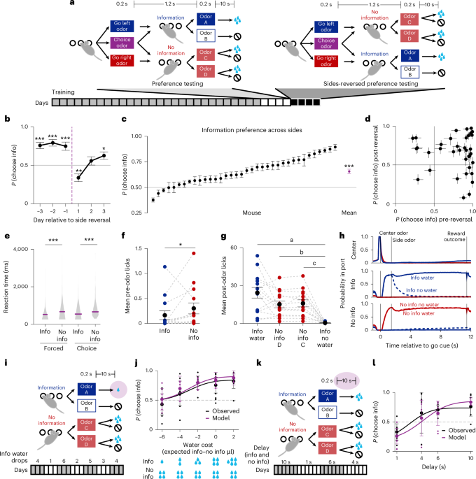
In the information seeking task, mice initiated trials by poking an illuminated center nosepoke port where one of three trial type odor cues was provided for 200 ms. Following a 50-ms 4,500-Hz go cue tone, the center port light went out and mice then chose either information or no information by poking into either the left or right reward port to trigger its infrared sensor. Each animal was initially assigned either left or right as the information port, pseudo-randomized across animals. Mice had to indicate their choice before the delivery of a 200-ms odor cue in the chosen side port 1.2 s after the completion of the go cue or the trial had to be repeated after allowing the remainder of its duration to elapse. On some training sessions, a grace period of up to 10 s was provided to extend the time available for the mouse to indicate its choice. In this case, the side odor was presented as soon as the mouse entered the correct side port. If mice did not stay in the center nosepoke for the duration of the center odor delivery and go cue, they were unable to proceed with the trial and had to repoke the center port for the full odor duration to proceed. After initial training (see details below), trials were of three types presented in pseudo-random order in blocks of 12: forced information, forced no information and choice. If mice chose the incorrect port on forced trials, they did not receive side port odor or reward and experienced an uncued timeout for the remainder of the full trial time and had to repeat the trial. These procedures ensured mice were unable to avoid nonpreferred trial types and equalized reward rates across trial types during training.

At the side ports, on each trial mice received one of four odors for 200 ms: the information port provided odor A on 25% of trials, which was always followed by water reward, or odor B on 75% of trials, which was never followed by a water reward. The no information port provided odor C on 75% of trials and odor D on 25% of trials, but the water reward was determined independently and provided on 25% of no information trials. The unequal frequency of odors C and D was designed to control for possible frequency effects on the neural representations of the side port odors A and B unassociated with their prediction of water value. The delivery of the side odor was followed by a delay period of 10 s in the main task. A 4,000-Hz 200-ms tone then indicated the outcome time on all trials, although water was only provided at that time on rewarded trials. Water rewards in the main task were 16 µl provided as 4 × 4 µl drops 50 ms apart. Unrewarded trials provided a time delay to match the duration of water delivery. The reward outcome period was followed by a 3-s intertrial interval. Mice were required to be present in the chosen port for water to be delivered, but they were not otherwise required to be in the port after indicating their choice.

All odors used in the task were monomolecular neutral odorants diluted in mineral oil, through which compressed medical-grade air was bubbled in custom-built olfactometers using mass flow controllers (Aalborg, GFCS-010201) and solenoid valves (The Lee Company, LHQA1221220H), whose opening was controlled by the Bpod system valve modules. Each odor bottle had a valve located before and after it to ensure accurate odor delivery timing. An odor line of 333 ml min−1 was combined with a carrier line of 333 ml min−1 to deliver a total air flow rate of approximately 667 ml min−1 into each of the three nosepoke ports. Air flow was maintained at the same rate but passed through a mineral oil control when odor stimuli were not being delivered. Odor identities were randomized across animals among four odors able to be delivered to the center port and four odors able to be delivered to either side port. Latch valves (The Lee Company, LHLA1221211H) switched odor delivery across the left and right sides. Odors were obtained at >98% purity from Sigma-Aldrich. Odors and concentrations used were as follows, at the center port: isoamyl acetate (1:10), pinene (1:5), benzaldehyde (1:10), limonene (1:5); at the side port: ethyl butyrate (1:20), acetophenone (1:5), octanal (1:5), cis-3-hexen-1-ol (1:10).

Behavior and olfactometer hardware were controlled by Bpod microcontroller systems (Sanworks, Finite State Machine r2.5) and their MATLAB interface as well as custom MATLAB code (Mathworks). Behavioral timestamps, video recording and imaging frame acquisition were synchronized using external data acquisition systems (National Instruments, USB-6002).

Behavioral training

Mice were trained to perform the information seeking task over several weeks of behavioral shaping progressing through the following stages.

1.

Covered side training (Extended Data Fig. 1a). Mice performed alternating blocks of trials where they had to trigger the center port and then enter the left or right port where they received water reward. The incorrect port was covered to prevent entry for the duration of each block of ~50 trials (200 µl total reward) each. Trials provided one to two drops of 4 µl of water, with the reward on the two sides being equal. The center port odors that would direct mice to each side on later forced trials were presented for the duration of the mouse’s triggering of the center port, and the duration of the center poke required to trigger the start of the trial was gradually increased to 200 ms. Delivery of water at the side port was delayed up to 1 s with gradual increases as mice became proficient at this training stage. The 3-s intertrial interval was also introduced to decrease repetitive behavior. Mice progressed to the next training stage when they achieved >50% complete trial initiations (remaining for the full 200 ms of center port odor presentation) and had rapid reaction times (<2 s).

2.

Uncovered side training (Extended Data Fig. 1b). This stage was not always included but was implemented for animals that had not fully learned the association between center port odors and the required forced side location. Mice completed blocks of ~20–50 trials directed to the left or right side by the odor provided in the center port with the incorrect side uncovered and accessible. They only received water if they chose the correct side port.

3.

Delay training (Extended Data Fig. 1b). Mice next performed trials with all ports uncovered and pseudo-randomly alternating forced left and right trials with the center port odor directing them to the left or the right. All correctly chosen trials were rewarded (one to two 4 µl drops) equally on the two sides. The delay between the completion of trial initiation at the center port and water reward delivery following correct choice of the side port was gradually increased by 200–1,000 ms approximately every 50 trials until the full delay value of 10 s was reached. Delays were increased manually while observing mouse behavior to moderate task difficulty and ensure animals maintained adequate motivation. During this stage, a reaction time requirement was instituted such that mice must choose the correct port within a certain amount of time to receive reward. This time was gradually decreased to the final value of 1.2 s. Mice moved on to the next training stage when they achieved >70% correct performance at the full delay value.

4.

Introduction of information (Extended Data Fig. 1c). In the next stage, trial rewards became probabilistic, and side port odors were introduced. Reward probability was decreased to 50% on all trials. Two hundred milisecond presentations of the side port odors (A, B, C and D) occurred 1.2 s after the go cue in the correctly chosen side port with the appropriate contingencies, such that odor A was always followed by water reward, odor B was never rewarded and odors C and D were each followed by water reward on 50% of trials. This allowed mice to begin learning that A and B resolved the trial’s outcome and provided information, while C and D did not provide information. Two to three sessions were performed at 50% reward and then the reward probability was dropped to 25%. Licking responses and the mouse’s presence in the reward port were monitored to ensure they were learning the meanings of the side port odors (mice tended to leave the side port following receipt of odor B). This training stage lasted five to seven sessions to ensure all mice learned that information was provided.

5.

Choice training (Extended Data Fig. 1d). Mice were explicitly taught that the choice center port odor allowed them to receive equal probability water reward at either side port in this stage of training. Task event times, side port odors and reward probabilities were the same as in the previous stage. Mice performed blocks of 10–50 trials with one side port covered to prevent accessing it. Trials with the appropriate forced odor (Information or No Information) for the uncovered side were alternated pseudo-randomly with trials in which the new choice odor was presented at the center port. Blocks were alternated to ensure mice experienced equal reward rates and total reward amounts following the choice odor on the left and right side to minimize side bias. This stage lasted for five to seven sessions, or ~250–300 choice trials on each side.

6.

Full task/preference measurement (Fig. 1a). Following choice training, mice were tested for preference for information on the full version of the task. Both side ports were uncovered and mice performed all three trial types: forced information, forced no information and choice, pseudo-randomly interleaved throughout each session. Trial types were set in blocks of 12 to ensure mice performed roughly equal numbers of trials of each type within a session, and rewards were assigned in blocks of 8 since trials were rewarded with 25% probability to ensure mice were rewarded frequently enough to maintain their motivation to engage in the task. In initial behavioral tests (n = 14), preference was tested for three sessions, then the side identities were reversed. Some mice (n = 7) performed two additional side reversals such that their preference was tested with information twice on each side for three sessions. In mice that were imaged and subsequent mice (n = 15), preference was tested for 6 days on each side to ensure stabilized learning of the relevant neural representations. On side reversals, the side locations of the information and no information side port odors were switched while center port odors still indicated movement to the same side. This meant that the center port odor that had previously signaled Information on the left side and was followed by odor A or odor B now signaled No information on the left side and was followed by odor C or odor D. Similarly, mice had to learn that Information had moved from the right to the left side or vice versa.

Water and delay titration experiments

Following side reversals, information was returned to the initial side port and mice were trained for several more sessions (~3) until their preference restabilized. Mice that had displayed information preference on both sides were then tested as follows in water (N = 4) and/or delay titration (N = 6) experiments (Fig. 1i–l). A stairstep procedure was used to determine the willingness of mice to sacrifice water reward for information. The reward probability on both sides was raised to 50%, but the reward amount on the information side was changed for 3 sessions at a time. Reward values of 4-µl drops were one drop, six drops, two drops, five drops, three drops and four drops, and then these amounts were retested in reverse order. Preference was calculated as the mean across the final session in each block at a given reward amount, such that two sessions were used to calculate the preference at each reward amount. Sessions with six drops were omitted from plotting and modeling due to ceiling effects. A similar procedure, but for single blocks of 6 days at each value, was used for imaged mice.

Information preference was measured across different durations of the delay between side odor presentation and water reward using a similar procedure in which preference was tested for 6 days at each delay value: 1 s, 10 s, 4 s, 10 s and 6 s. Preference was determined as the mean preference for information in the last two sessions at each delay value.

Task with reward cues on all trials

The task was modified to explicitly cue mice when reward would be revealed so that they learned they could leave the side port on all trials (Extended Data Fig. 2). In all stages of this training, after mice experienced 80% of the delay length between the side port odor delivery (or in earlier stages, their entry into the side port) and the reward outcome, the correctly chosen reward port illuminated and a tone played for 50 ms to indicate whether that trial would be rewarded. This then gave mice 2 s at full delay to return to the reward port and collect water. A 500-Hz tone indicated a rewarded trial, while a 2,000-Hz tone indicated an unrewarded trial.

Task with four information- and water-predicting CS odors at the center port

Five mice with completed surgery for OFC imaging that had been previously trained on the information seeking task and had strong information preference were trained on this additional task (Fig. 3d). First, mice were trained to follow the ‘high water value’ odor to one side port and receive 8 × 4-µl drops of water and the ‘low water value’ odor to the other side to receive 2 × 4-µl drops of water. The side that had previously been the preferred information side was assigned as the small water side. One side port was covered and mice performed blocks of trials on one side, then the other. Then these two large and small water trial types were pseudo-randomly interleaved with all ports uncovered. Owing to limitations in the olfactometer, which could only provide four odors at the center port, the odor that had previously indicated free choice trials became the ‘small water’ odor and the fourth odor that had not previously been used was the ‘large water’ odor. Mice performed seven to ten training sessions in this stage. Mice then performed one to three sessions of interleaved forced information and forced no information trials as they had learned earlier in the main task version. Mice then performed the full version of this task with information, no information, large water and small water trials pseudo-randomly interleaved in blocks of eight to ensure adequate exposure to all trial types. Mice performed six sessions with the sides in the initial configuration followed by six sessions with the side identities reversed. Information and low water value were assigned to the same side port, while no information and high water value were assigned to the other.

Licks

Licks were recorded in initial behavioral sessions (N = 14 mice) using capacitance sensors (Phidgets, 1129_1B) at each port’s lick spout.

Stereotactic surgery

Mice were anesthetized with ketamine (100 mg kg−1) and xylazine (10 mg kg−1) through intraperitoneal injection and received analgesia via buprenorphine sustained-release subcutaneous injection (0.75 mg kg−1) and carprofen (3 mg kg−1), had fur shaved from their head and then were placed in a stereotactic frame. Body temperature was maintained using a heating pad attached to a temperature controller. For lens implantation experiments, a 1.1–1.5-mm round craniotomy centered on the implantation coordinates was made using a dental drill. The dura was removed and <0.1 mm of tissue aspirated, and 0.3 µl GCaMP6f virus (AAV1.CaMK2a.GCaMP6f.WPRE. bGHpA, 3.35 × 1012 vG ml−1, Inscopix) was injected into lateral OFC (medial-lateral (ML), 1.0; anterior-posterior (AP), 2.4; dorsal-ventral (DV), 2.45 mm from Bregma) at ~50 nl min−1 using a pulled micropipette. After allowing the virus to diffuse undisturbed for 5 min, the needle was removed and a 0.5-mm or 1-mm diameter and 4.0-mm length microendoscope GRIN lens with integrated baseplate (Inscopix) was then inserted at a depth just above the injection site and centered over it (ML, 1.0; AP, 2.4; DV, 2.4 mm from Bregma). The combined lens and microscope baseplate assembly (Inscopix) was secured to the skull using Metabond (Parkell) and further secured and covered with black dental cement (Ortho Jet). Mice recovered for at least 1 week before the beginning of water restriction and behavioral training.

Histology

Mice were euthanized after anesthesia with ketamine/xylazine by perfusion with 4% paraformaldehyde. Brain tissue was removed for 24 h fixation, and coronal sections (120 µm) were cut on a vibratome (Leica). The sections were incubated with far-red neurotrace (640/660, Thermo Fisher Scientific) to label neuronal cell bodies. Images were collected using a Zeiss LSM-710 confocal microscope system. Histology was performed to confirm locations of implanted lenses, as well as expression levels for GCaMP using native fluorescence.

Imaging experiments

Seven mice were imaged throughout the course of training and testing in the main task, including during 10-s and 1-s delay sessions (Supplementary Tables 3–7). Five additional mice were imaged throughout learning and performance of the four-odor center port information and water prediction task (Supplementary Table 8). Recordings of GCaMP activity were made using Inscopix miniaturized microscopes (nVista3.0) with commutators used in passive mode, with uncompressed videos saved using the Inscopix system. Before being placed in the behavior chamber, awake mice had the miniature microscope (Inscopix) attached securely to their skull baseplate. Neural activity was then recorded throughout the behavior session (50–100 min) and the microscope was removed and the baseplate cover reattached. Images were recorded with the lowest possible LED illumination to visualize calcium transients with settings largely preserved from session-to-session within each animal. Generally, LED power was set between 0.3 and 1 mW, with most animals remaining <0.7 mW. The z focus of the microscope was adjusted rarely to maintain the same field of view based on landmarks such as blood vessels.

Quantification and statistical analysis

No statistical method was used to predetermine sample sizes. All mice that completed training during water restriction with adequate weight maintained and that displayed the expected differences in reward port occupancy based on the predicted water reward were included in preference testing and shown in Fig. 1b–e. Less than 15% of mice failed to learn the task by this criterion. Mice that displayed information preference on both the left and the right side were used for water and delay titration and imaging experiments given that these experiments were designed to test the effect of increases in information cost and decreases in information value on information preference. Both male and female mice were used, information preference data are reported disaggregated, and no difference was observed. Blinding of experimenters to conditions was not applicable. Information side and odors were pseudo-randomly assigned across animals.

Statistical tests are indicated in the text and/or figure legends. Nonparametric tests were used unless otherwise described. Tests are two tailed unless otherwise noted. Exact P values are given, except for when below the level of computer precision or in permutation tests, when the observed value exceeded all permutations.

Behavior analysis

Behavior was analyzed using custom MATLAB scripts. Mice performed approximately 150 trials per session. We examined information preference on free choice trials across all of the preference testing sessions (‘overall preference’; Fig. 1c) or in the last 200 free choice trials prior to the first side reversal and the last 200 trials after reversal before either ending preference testing, reversing the sides again or progressing to delay or reward amount manipulations. For most animals, these 200 trials occurred in the last 3 days before and after reversal, since mice performed around 50–60 choice trials per session. Extended Data Fig. 1j shows pre-reversal preference in these 200 choice trials and Fig. 1d shows preference before and after reversal. Since choice preference is the probability of the binary outcome of choosing information or no information, we used MATLAB’s binofit function to estimate the information choice probability, P(info), and 95% CIs for each animal. We then tested whether the means of these values across animals were different from 50% (indifference) using two-sided sign rank tests (MATLAB signrank). We fit a generalized linear regression model to compute coefficients for the correlation of side and information with choice for each animal using MATLAB’s glmfit function for binomial data with the default ‘logit’ link function (Extended Data Fig. 1l). These coefficients provide the ‘log odds’ influence of side and information on choice.

We also estimated the probability of correct choice on forced trials using binofit and report data across animals in the same way as preference. For reward rate, licks and probability of poking in nose ports, we report the mean across sessions per animal and computed the population mean and standard error. Reaction time is the time elapsed from the go cue until the first entry of the correctly chosen side port and is reported per-trial by trial type. Reward rate is calculated as the mean water amount received per minute of correct trials. The probability in port is shown as either the mean across the delay between the end of the side port odor stimulus and the reward outcome or the mean across the first 1 s after the end of the side port odor stimulus. On plots showing the full trial duration (Fig. 1h and Extended Data Fig. 2d), the trial is binned into 50-ms increments to compute the probability of being in a particular port. In contrast to the correlation we identified between information preference and reaction time (Extended Data Fig. 1n), we did not detect correlations between information preference and time spent in the information versus no information port, licking before receipt of the side port odor or licking following information odor A (water) and information odor B (no water).

Unless otherwise indicated, behavioral data are from the last three sessions before the first side reversal. Before pooling data across sessions, we confirmed that there were not significant cross-session differences using a nonparametric within-subjects design (Friedman’s ANOVA with Tukey–Kramer correction for multiple comparison).

Behavioral models

Cognitive decision models, fit to single trial level-choice data, have been used in neuroscience and behavioral economics for decades to provide evidence that a specific type of computation may be underlying choice trends seen in a given dataset71. The two main questions we sought to answer with decision model frameworks here were (1) ‘why do information-preferring mice not always choose information?’ and (2) ‘can the observed experimental behavioral trends be explained by a model that uses separate but interacting reinforcement learning (RL) machinery for processing traditional water rewards and intrinsic information rewards?’. We hypothesized that there is an interaction between RL-like computations of information value and water value following recent literature21 and used a list of relevant models of increasing complexity to test this hypothesis.

In decision model literature, there are a large variety of RL-related models, often becoming quite complex, which risks over-parametrization and over-fitting if the number of agents fit and task complexity do not scale with the model complexity72,73. Thus, for the purposes and constraints of this study, we chose to use the simplest implementation of RL computations, the Rescorla–Wagner model, following similar recent related work in human models40. The models tested are outlined below and incrementally built up to the full model that contains the minimal necessary components to explain both the water-tuning and delay-tuning experiments (Fig. 1j,l and Extended Data Fig. 3). The MATLAB package fitPsycheCurveWH was used to fit a psychometric curve to each mouse’s real choices as well as the predicted choices from each of the models tested, using the best parameter initializations from a grid search.

First, all models tested transform a decision variable DV term, which summarizes the core computation, into a sigmoid-transformed binary choice probability \({P(t)}_{\rm{info}}\), here the probability of choosing information at trial t

$$P{(t)}_{\mathrm{info}}\,=\frac{1}{1\,+\,{e}^{[-DV(t)]}}$$

(1)

The term \({P(t)}_{\rm{info}}\) is optimized through a negative log likelihood minimization

$${\rm{NLL}}=-\mathop{\sum }\limits_{t=1}^{{n}{\rm{Trials}}}\left\{\log \left({P\left(t\right)}_{\rm{info}}\right){C\left(t\right)}_{\rm{info}}+\log \left({1-P\left(t\right)}_{\rm{info}}\right)\left(1-{C\left(t\right)}_{\rm{info}}\right)\right\}$$

(2)

where is \({C(t)}_{\rm{info}}\) = 1 for an information choice and 0 for a noninformation choice. Models were each run with 16 initializations of different starting parameter values and numerically solved using the fminsearchbnd function in MATLAB using a grid search of parameter windows. The nature of DV(t) changes in each model, as summarized below

RL water model

$${\rm{DV}}\left(t\right)=\frac{1}{\sigma }\left\{\beta \Delta Q\left(t\right)+\varepsilon \right\}$$

(3)

The time-independent fit parameters are \(\sigma\), the normalization constant (inverse temperature), \(\beta\), a relative weight factor for the traditional Rescorla–Wagner RL term of water \(\Delta Q\left(t\right)\) and \(\varepsilon\), a bias term, which allows for a flat baseline tendency toward or away from choosing information that the water term is weighted against. The time-dependent term \(\Delta Q\left(t\right)\) is defined as the difference of the value functions for the information and no-information sides of the task as usual in binary choice tasks

$$\Delta Q\left(t\right)={Q(t)}_{\rm{info}}-{Q(t)}_{\rm{no}-{\rm{info}}}$$

(4)

Each \({Q(t)}_{i}\) for i = info, no info is defined according to the Rescorla–Wagner equation with learning rate \({\alpha }_{1}\) and prediction error \(\delta (t)\) when choice i is chosen

$${Q(t)}_{i}={Q(t-1)}_{i}+\,{\alpha }_{1}{\delta (t)}_{i}$$

(5)

$${\delta (t)}_{i}={{{\rm{Reward}}\left(t-1\right)}_{i}-Q(t-1)}_{i}$$

(6)

When a choice is not chosen, with unchosen choice j, then \({Q(t)}_{j}={Q(t-1)}_{j}.\)

The next model tested contains only information-related terms with a new Rescorla–Wagner term \(S\left(t\right)\) for information value with information prediction error \(\theta \left(t\right)\) and learning rate \({\alpha }_{2}\), following analogous logic to recent nontraditional RL equations such as choice prediction errors74

λ-RLinfo model

$$\begin{array}{c}{\rm{DV}}\left(t\right)=\frac{1}{\sigma }\left\{S\left(t\right)+\varepsilon \right\}\,\\ S(t)=S(t-1)+\,{\alpha }_{2}\theta (t)\\ \theta \left(t\right)=\left\{{\left(\frac{{\rm{Delay}}(t-1)}{10{\rm{s}}}\right)}^{\lambda }-S(t-1)\right\}{\rm{if}}\;{\rm{info}}\;{\rm{is}}\;{\rm{chosen}}\\ \theta \left(t\right)=\left\{0-S(t-1)\right\}{\rm{if}}\;{\rm{noinfo}}\;{\rm{is}}\;{\rm{chosen}}\,\end{array}$$

(7)

Thus, information’s ‘value’ is \({\left(\frac{10{\rm{s}}}{10{\rm{s}}}\right)}^{\lambda }=1\) for the maximum delay of 10 s, but then is exponentially discounted as delay decreases, following the strong tendency observed in the mice data. When the mice do not choose information, they receive no information value and thus the info-reward is set to zero.

The next model tries to remove the λ decay exponent, but combine the RLwater term with the RLinfo term simplified to have λ = 0, so that information value = 1 on information choices regardless of delay length.

RLwater + RLinfo model

$${\rm{DV}}\left(t\right)=\frac{1}{\sigma }\left\{{\beta \Delta Q\left(t\right)+S\left(t\right)}_{\lambda =0}+\varepsilon \right\}$$

(8)

Then, the full model combining both water value and exponential delay-modulated information value computations is defined below, conceptually motivated by recent work finding both types of value are processed in an interacting way21.

RLwater + λ-RLinfo model:

$${\rm{DV}}\left(t\right)=\frac{1}{\sigma }\left\{\beta \Delta Q\left(t\right)+S\left(t\right)+\varepsilon \right\}$$

(9)

As an alternative to exponential modulation of the information value by the delay length, we also tested a hyperbolic variant of equation (7), replacing \({(\frac{{\rm{Delay}}(t-1)}{10{\rm{s}}})}^{\lambda }\) with a hyperbolic term \(0.5{(1-\kappa\frac{{\rm{Delay}}\left(t-1\right)}{10{\rm{s}}})}^{-1}\)

RLwater + λ-RLinfo model (hyperbolic)

$${\rm{DV}}\left(t\right)=\frac{1}{\sigma }\left\{{\beta \Delta Q\left(t\right)+S\left(t\right)}_{\kappa }+\varepsilon \right\}$$

(10)

Last, as a conceptually alternative decision model, we made a weighted win-stay lose-shift (WS-LS) model, that regressed the past trial information and reward conditions to predict the current choice

WS-LS model

$$\begin{array}{l}{\rm{DV}}\left(t\right)=\frac{1}{\sigma }\left\{{\beta }_{1}{\rm{InfoRew}}\left(t-1\right)+{\beta }_{2}{\rm{NoInfoRew}}\left(t-1\right)\right.\\\quad\quad\quad\,\,\,\,\,\,\left.+{\beta }_{3}{\rm{InfoNoRew}}\left(t-1\right)+{\beta }_{4} {\rm{NoInfoNoRew}}\left(t-1\right)+\varepsilon \right\}\end{array}$$

(11)

Each \({\beta }_{i}\) condition variable is either 0 or 1. For example, Info No Rew = 1 if the past trial was an unrewarded information choice (either forced or choice), but 0 otherwise.

The total number of mice fit was N = 10 for all models, but for 4/10 mice only the water tuning data was fit, not the delay-tuning data since those mice did not perform delay-tuned task variants. These mice have had their \(\lambda\) discount exponent removed as shown in Supplementary Table 9 of fit parameters. Then 4/10 mice did not have water tuning data fit. These mice have all fit parameters in Supplementary Table 9. To show the data were not overfit, each model was fit five times with different randomized 67% train versus 33% test splits per model for cross-validation (Supplementary Table 10). Mean and standard deviation of normalized AIC and accuracy are shown in the table across the five runs.

To see how much each RL component improved the full model fit, the average Akaike information criterion (AIC) was calculated according to the standard equation for each model, with k as the number of free parameters75

$${\rm{AIC}}=2k+{2}{\rm{NLL}}$$

(12)

The full RLwater + λ-RLinfo model is shown in Fig. 1. The auxiliary models are presented in Extended Data Fig. 3. It is visually clear that only the RLwater + λ-RLinfo can simultaneously capture the important trends from the data in both water tuning and delay-tuning experiments. Future work seeking to do more advanced decision modeling with further corrections to the Rescorla–Wagner formulation should increase the sample size and tune a wider range of experimental conditions, but the current models implemented show that the minimally simple RL formulation that accounts for both water value and information value is able to explain the full range of experimental conditions tested here. As a caveat, we do not claim our fitted parameters are unique or will work for all future studies, a common issue in cognitive decision models because model parameter magnitudes and scaling are not independent and thus degenerate solutions probably exist71,72. However, this well-known issue does not undermine the finding that the minimal two-value-type RL model machinery performs well in our context.

Imaging data processing

Raw video data were spatially downsampled at 4× and saved as Tiff files using the Inscopix Python API. We used the NormCorre rigid motion algorithm76 to both remove movement artifacts from imaging videos and to align the field of view across sessions to facilitate cell registration. We motion corrected videos filtered to reveal more stationary landmarks such as blood vessels and then applied the computed X–Y shifts to the original videos. To filter videos, we took a difference of Gaussians approach to extract potential stationary features smaller than cell diameter from the larger background fluctuation. We applied a Gaussian filter (Matlab imgaussfilt) with a radius of 2 to our downsampled 200 × 320 pixel images and subtracted pixel values of the images separately filtered with a larger radius (MATLAB imgaussfilt radius 6). We then set a threshold value of 4 and set all pixel values less than this threshold to its value. This resulted in a filtered video with mostly black background and light-to-white landmarks on which we performed motion correction and generated a mean template image.

Motion correction was performed within each session using the NormCorre algorithm using the following parameters: ‘bin_width’ 500, ‘init_batch’ 1,000, ‘max_shift’ 10, ‘iter’ 2. We then used NormCorre to align each session’s video frame-by-frame to the filtered template from a central ‘anchor’ session for each animal (typically the final day of preference testing before the first side reversal). The alignment of the template field of view from each session was manually inspected to ensure accurate registration across sessions. Cell location footprints and activity were then extracted using the MATLAB implementation of CNMF-E77 as follows.

CNMF-E default parameters were used, except that min_corr and min_pnr were adjusted for each animal to maximize cells identified during the initialized step of the algorithm (min_corr range 0.7–0.8, min_pnr 8–10) and gSig = 3, gSiz = 11. For initialization, min_pixel was set to 25 and for identification of cells in the residual after background subtraction, min_corr_res = 0.8 and min_pnr_res = 9. Following two iterations of CNMF-E’s cell footprint and calcium activity extraction, we applied several additional filters to remove false positives, taken from the incorporation of the CNMF-E algorithm into the Caiman Python implementation78. We set thresholds for temporal sparseness, minimum peak-to-noise and a constant baseline of activity. We first removed cells with temporal sparsity <0.003.

$$\begin{array}{l}{\rm{Temporal}}\,{\rm{sparsity}}\\={\rm{sqrt}}({\rm{sum}}({\rm{neuron}}.{\rm{C}}\_{\rm{raw}}.^\wedge\mathrm{2,2}))./{\rm{sum}}({\rm{abs}}({\rm{neuron}}.{\rm{C\_raw}}),\,2)\end{array}$$

(13)

We then removed cells with peak_to_noise_ratio <8.5

$${\rm{PNR}}=\max ({\rm{neuron}}.{\rm{C}},[],2)./{\rm{std}}({\rm{neuron}}.{\rm{C\_raw}}-{\rm{neuron}}.{\rm{C}},\,0,\,2)$$

(14)

Finally, we removed cells in which CNMF-E’s detrending of the calcium fluorescence across the session was ineffective and that had large differences in the baseline fluorescence between the beginning and end of the session. We computed the difference from baseline by taking the difference in mean activity between the first and last 10% of the session frames and removed cells for which this absolute value was greater than 3.

$$\begin{array}{l}{\rm{difference\_from\_baseline}}={\rm{mean}}({\rm{neuron}}.\\{\rm{C}}\_{\rm{raw}}(:,1:{\rm{round}}(0.1^*{\rm{size}}({\rm{neuron}}.{\rm{C\_raw}},2))),\\2)-{\rm{mean}}({\rm{neuron}}.{\rm{C\_raw}}(:,{\rm{end}}-{\rm{round}}\\(0.1^* {\rm{size}}({\rm{neuron}}.{\rm{C\_raw}},2)):{\rm{end}}),2)\end{array}$$

(15)

We then visually inspected each cell using CNMF-E’s viewNeurons method to ensure appropriate neuron-like shape and calcium transients and removed false positive cell identifications.

Using this procedure, we were able to register cell spatial footprints across sessions several weeks apart, over the entire months-long course of training, for up to four sessions simultaneously using the register_multisession function from the MATLAB implementation of CaImAn78. We used the default parameters for register_multisession, with the exception of setting the threshold for turning spatial components into binary masks, options.dist_maxthr = 0.22, and the threshold for setting a distance to infinity, options.dist_thr = 0.6. Cell registration fidelity between individual sessions was visually inspected using the register_ROIS method for maximum overlap and false positives to appropriately set parameters. For 4/5 mice imaged in the four center port odor information and water value prediction task, a newer algorithm, SCOUT, was used to register cells. SCOUT registration of cells used the default parameters79.

Analysis of neural activity

We used the calcium signal, C, output by CNMF-E that is smoothed with a kernel based on the time course of GCaMP6f signal decay as the calcium activity, a proxy reflecting neural spiking activity, of each cell across each session. As CNMF-E subtracts the background signal from each imaged frame individually, the output activity, C, may be considered a scaled version of the change in fluorescence over background (ΔF/F) at each frame. Moreover, given this background subtraction, this signal is already normalized77. We therefore analyzed and report raw ‘calcium activity’. We also tested a standard z-score normalization procedure subtracting each cell’s mean across each session and dividing by the standard deviation, and this did not qualitatively affect the results.

Neural activity in each session was aligned to behavioral events using DAQ timestamps, and we analyzed neural activity across all mice considering cells across animals as a single pool for single-cell analyses, except where otherwise noted. Our CEBRA model simultaneously fit across animals using all cells, not just those registered day to day, with the same qualitative findings about information and water value encoding supports pooling cells across animals. The main dataset (Supplementary Table 3) consisted of cells registered across four sessions surrounding a side reversal such that there were two sessions with information on each side (left and right), with 56–216 cells per animal across seven animals (N = 1,138 total neurons). Datasets for delay comparisons (10 s versus 1 s; Supplementary Tables 5–7) and learning (Supplementary Table 4) also consisted of four sessions per animal across six and seven animals, respectively, with similar numbers of cells per animal (N = 992 total delay neurons, 788 total learning neurons). Data for mice imaged in the four-odor center port information and water value prediction task involved cells registered across four sessions surrounding a left–right side reversal, with 964 cells from five animals (Supplementary Table 8).

All analyses of neural activity used correct forced trials, except those of Fig. 3c,h and Extended Data Fig. 6a–d,g, which used choice trials. Analyses of the main dataset and four CS center odor task balanced left and right side trials by matching sessions across side reversal thus approximately equalizing the number of correct forced information and no information trials on each side given the pseudo-random block trial structure for the calculation of coding indices (below) and mean activity. Decoding analyses precisely balanced trials across sides (details below). Analyses across task learning and information value manipulations necessarily used data with information on a single side.

We computed indices of cross-validated differential activity to analyze OFC neurons’ encoding of task variables (coding index). For each pair of conditions (for example, information and no information) within each neuron, we balanced (cross-validated) the direction of the difference in activity (that is, sign). We multiplied the mean difference in activity between the two conditions for one arbitrary half of the trials (for example, even-numbered trials) by the sign of the mean difference on the other half of the trials (for example, odd-numbered trials) and vice versa, and then took the mean value of these two split halves as the coding index for that cell

$$\begin{array}{ll}{\rm{coding}}\,{\rm{index}}=({\rm{sign}}({\rm{activity}}\,{\rm{difference}}\,{\rm{in}}\,{\rm{OddTrials}})\,{\rm{x}}\\\qquad\qquad\qquad\,\,\,\,\,{\rm{activity}}\,{\rm{difference}}\,{\rm{in}}\,{\rm{EvenTrials}}+\\\qquad\qquad\qquad\,\,\,\,\,{\rm{sign}}({\rm{activitydifference}}\,{\rm{in}}\,{\rm{EvenTrials}})\,\\\qquad\qquad\qquad\,\,\,\,\,{\rm{x}}\,{\rm{activitydifference}}\,{\rm{in\; OddTrials}})* 0.5\end{array}$$

(16)

This procedure is similar to taking the absolute value of the difference in activity but instead creates an index of differential activity centered at zero in the absence of consistently greater activity in a particular condition. We then averaged these indices to find the coding index across the population.

We computed the coding indices across the full trial time course at each imaged frame, beginning at the onset of center port odor on the mouse’s center port entry that successfully initiated the trial. Mice sometimes entered the center port and received a partial odor stimulus prior to successfully initiating a trial by remaining in the port through the completion of the go cue tone, which may have meant that OFC responded differently at the animal’s first and subsequent center port odor presentations. Thus, we computed full-trial coding indices surrounding the odor presentation at successful trial initiation, from which the remaining trial events proceeded.

To analyze neural responses and identify CS and US value representations at specific trial epochs, we examined coding indices in a 1-s window following each trial event: the first center port odor presentation, the side port odor presentation and the reward outcome. We determined the 1-s post-event activity window by observing the raw odor responses and peak differential activity around each event in our task. We also determined the time course of odor stimulus delivery in the nosepoke ports using a photoionization detector (Aurora Scientific, 200b miniPID). Although we observed small differences in the timing of odor availability, on average odor was first detectable 0.075 s after odor valves were open and peaked at 250 ms after valve opening. The neural responses we observed peaked within 1 s of odor onset. We have therefore used a window of 0.2–1.2 s after the timing of events recorded by our Bpod system (odor and water valve opening), and a comparable window 1.2–0.2 s before events, to analyze neural responses. For plot visualizations, we have indicated odor onsets 0.075 s after the opening of the odor valves in the olfactometer.

To determine whether cells, and the OFC population on average, encoded differential activity between two conditions as computed in our coding index in a task epoch, we took a bootstrapping approach. We compared the difference in the mean coding index in the 1 s window after an event to the mean index in the 1 s window before it to account for the fact that activity continuously varied throughout the task and, in particular, was often already elevated just before the side port odor delivery. Thus, for a given set of conditions (for example, information and no information), we shuffled trials between the two conditions 1,000 times. For each shuffle, we determined the difference between the mean coding index in the 1-s window after the trial event and the mean coding index in the 1-s window before the trial event. We then determined the percentage of these shuffled values that were less than the observed increase in differential activity to estimate the statistical likelihood of the observed difference (P value). We defined a cell as contributing to a representation or encoding a difference between conditions if the observed coding index difference was greater than that of at least 5% of shuffled data. Similarly, we defined that the OFC population encodes a difference between conditions if the mean population coding index difference around an event was greater than 95% of the shuffled values. Extended Data Fig. 5b–e shows the event-specific coding indices we computed in addition to the full trial information and water coding indices.

We performed a shuffling procedure to evaluate the statistical significance of the different correlation values for the data in Fig. 3h,i. Under the null hypothesis that these two datasets come from a common underlying distribution, we combined all the data points in these two figures and randomly assigned them to two groups, with the number of points in each group matching the numbers in the figures. We then computed the ratio of correlation coefficients for these two random groups. We repeated this for 100,000 random shuffles and report the fraction of shuffles for which the ratio was greater than or equal to that of the data.

Cells with significant conditional responses to task events (responding cells)

Cells were identified as responding to an event in a task condition using a rank-sum test to determine if their activity in the post-event 1-s period (as above) in that condition was different from activity in the pre-event 1-s period in that condition, which we considered the baseline activity for that event. To accommodate baseline activity that was already elevated due to earlier trial events given the close proximity in time of the center and side port odors, we determined the maximum activity for each cell on each trial in the pre-event period and fit an exponential decay function based on GCaMP6f fluorescence (λ = 4) to determine its predicted activity in the post-stimulus period. If the absolute value of difference between the mean of that predicted activity in the post-event period and the mean of the observed activity in the post-event period on that trial was greater than 0.2, the GCaMP fluorescence-predicted activity in the post-event period was used as the baseline. If not, the pre-event activity served as the baseline. Cells with significant responses were then identified as those in that condition with mean activity in the post-event period significantly greater than baseline using a rank-sum test and with the value of that difference greater than 0.1. This procedure offers a conservative identification of responding cells to prevent false positives. Using a more standard procedure with a rank-sum test on mean activity before and after the event falsely identified many cells with delayed responses to the center port odor whose activity then diminished as expected for calcium signals at the same time as the side port odor delivery as ‘responding’ to the side port odor. We therefore used the above approach to more conservatively identify cells with activity changes due to the side port odor.

Mean activity

For plots showing population mean activity, each cell’s mean activity on the indicated trial type was calculated, its mean activity within the 1-s pre-event window was subtracted and then all cells’ mean activities were averaged. Single-cell plots are shown with the mean activity in the 1-s pre-event window subtracted. To test whether the population mean responses to center port odors changed across delay changes and learning (Extended Data Fig. 8a,k), we compared the mean activity in the 1-s window after the center port odor across all trials between the two conditions, using a rank-sum test for significance.

Heat maps

Population calcium activity and coding index heat map plots display the mean activity or coding index for each cell across trials in each condition. Heat maps of mean calcium activity, and not those of differential activity using coding indices or activity differences, have the cell’s mean activity in that condition across the pre-event 1-s period subtracted for better visualization. Plots within panels are all sorted by the indicated activity such that a single cell can be read across the entire heat map.

Decoding

Linear classifiers based on support vector machine architecture were used to decode trial types using the Decodanda Python package (https://github.com/lposani/decodanda)80. Decodanda uses the Python package scikit-learn to implement support vector machines. Classification was performed on 200-ms bins of neural data, with calcium activity averaged for each cell on each trial within each bin or, for overall mean classification accuracy, on calcium activity averaged for each cell on each trial within the 1-s window following the center odor stimulus onset (post-event period). For decoding accuracy across bins of time in trials, analysis was performed separately for each time bin. Decoding performance was computed using 20-fold cross-validation, in which trials for each animal were split into samples for training (75% of trials) and testing (25%) sets at each fold. Decoding accuracy was taken as the mean across the 20 cross-validation folds. Trial samples were balanced across both information or water value conditions and left–right side across side reversals to eliminate confounding between possible side location and value encoding. Trials were either sampled from imaging sessions within a single animal or by pooling across animals. Pseudo-populations of cellular activity were generated by sampling an equal number of trials (N = 200) of each combination of conditions from each animal. For example, to decode information versus no information trials, in each cross-validation fold, each animal’s information left, information right, no information left and no information right trials were split into testing and training fractions. Then, 200 samples were taken from each set of conditions for training. These data are then pooled across animals. For decoding of free choice trials (information choice versus no information choice), only data from four of seven mice were used because the other three animals had fewer than four no information choice trials on one side due to high information preference. Accuracies were compared to the decoding accuracy obtained from a null model computed by randomly shuffling the labels of trials. For each decoding test, ten null model iterations were performed, and statistical significance of the performance accuracy of data decoding was determined by the one-tailed z score compared to the distribution of null model accuracies.

We determined the coding importance, \({w}_{i}^{x},\) of each cell for each classifier, following the method employed in ref. 80 For each variable, X, for each cell i, we computed the absolute value of the average decoding weight normalized by the standard deviation across validation folds, where n is the cross-validation fold

$${w}_{i}^{x}:=\left|\frac{{E\left[{w}_{i,n}^{x}\right]}_{n}}{\sigma {E\left[{w}_{i,n}^{x}\right]}_{n}}\right|$$

We then computed the Pearson correlation between these weights for the information versus no information and high versus low water value classifiers. We also computed the correlation between these weights for the information forced versus no information forced and information choice versus no information forced classifiers.

Principal component analysis to identify information–no information axis in population activity space

To compute an axis along the information–no information dimension in population activity space, we calculated the difference between the mean activity on correct information forced and the mean on correct no information forced trials for each cell following the center port odor presentation (0–0.8 s after odor valve opening) in our main dataset with two sessions with information on the left and two on the right side. We then computed the principal components of that population activity difference (MATLAB function svd). The first component captured >80% of the variance in this activity computed from the variance of the projection of the information and no information trial activity onto the first component divided by the total variance of activity on information and no information trials. We therefore projected the population activity in each trial, and the mean within each condition (information and no information), onto the first principal component for visualization.

CEBRA modeling

We used CEBRA to better understand how a complex task such as ours is represented at the neural level. The complexity of our task, together with the possibility that the OFC, as a frontal region, contains neural representations that are more compressed and processed compared to other regions, suggested that neural task representations are more likely to have arisen from the nonlinear combination of neural signals33,36. A nonlinear latent variable model such as CEBRA, unlike principal component analysis, for example, reduces the chance that an analysis is fitting task-irrelevant noise or missing important nonlinear signals that are crucial to accurately capture how a task is encoded at the population level.

More specifically, we used CEBRA to obtain low-dimensional task embeddings by jointly fitting neural data and task-relevant behavioral variables in a time-dependent manner. We generated time-stamped labels expressing task structure and mouse behavior, as further specified below, and fitted these together with the neural data by minimizing an InfoNCE contrastive loss objective53. We fit the model to the entire cohort of animals at once, such that contrastive samples were chosen from across all animals. We thus obtained latent embeddings that were informative and consistent across animals. We examined the geometry of the information and water value representations in the embeddings and measured the differences between these two representations over the course of each trial. We confirmed that the embeddings were informative by decoding task-relevant variables and comparing results to shuffled versions that scrambled the association of particular labels with the recordings.

We fit CEBRA models with the following specifications: model architecture = ‘offset1-model’, batch size = 1,024, distance = ‘cosine’, conditional = ‘time_delta’, temperature = ‘auto’, learning rate = 0.001, max iterations = 5,000, output dimension = 3, number hidden units = 100. We arrived at these settings by fitting CEBRA models on the data from three mice and picking the settings that achieved the lowest overall InfoNCE81 loss value after 10,000 iterations; during this process we observed that only half the iterations were necessary for the loss to converge so we set max iterations to 5,000 to minimize compute.

We fit two types of models which we refer to as full and delay. The full model is fit on data with a long delay (t_d_l = 10 s) between the side port odor and reward delivery, while the delay model is fit on data with both short (t_d_s = 1 s) and long delay (t_d_l = 10 s) and is aimed at embedding the two delay types in a joint space for comparison.

The full model was fit on six mice (JB432, JB426, JB434, JB413, JB424 and JB425) with cell and trial counts as specified below (Supplementary Table 11). Importantly, we employed a multisession setup in which each session with its unique dimensionality was added into the fitting process accompanied by shared context labels (Supplementary Table 13), which allowed CEBRA to learn a shared embedding space for signals from all sessions (across all mice). We used sessions from our main dataset balanced before and after information side reversal, such that each mouse was fit with two sessions with information on each side (left/right). To achieve an unbiased representation across all conditions, we equilibrated the number of trials across conditions such that there were equal numbers of trials across the four conditions resulting from the interaction of ‘reward versus no reward’ and ‘information versus no information’. For the full model, the number of time points per trial is fixed at n_time = 320 time points per trial throughout, ranging from the initiation of the last (if multiple) presentation of the center port odor all the way until after reward delivery.

The delay model was fit on six mice (JB432, JB433, JB434, JB426, JB424 and JB425) with cell and trial counts (Supplementary Table 12) and label types (Supplementary Table 13) with n_time = 113, as specified below. To make the two delay types (short and long delay) comparable, with identical context labels across sessions allowing sessions with variable cell counts to be fitted together in one model, we excerpted the outcome period in the long delay trials and concatenated it after the first ~1 s of the 10-s delay period (omitting most of the longer delay) thus making the overall duration of short and long delay trials the same. These sessions do not include a reversal of the information port location. As before, to achieve an unbiased representation across all conditions, we equilibrated the number of trials across conditions such that there were equal numbers of trials across the four conditions resulting from the interaction of ‘reward versus no reward’ and ‘information versus no information’; in case that resulted in less than one trial per condition, we equilibrated instead by ‘information versus no information’ only (session marked with * in Supplementary Table 12).

Unlike the full model, we matched cells across all recording sessions for a particular mouse before fitting the delay model (hence the matching cell counts in Supplementary Table 13). We then combined all of a mouse’s recording sessions into a single array and fitted the recordings and labels (Supplementary Table 11) with CEBRA in a single-session setup. This allowed us to derive a common embedding space across both delay types.

We fit all CEBRA models on the neural data (as defined above) together with the specified label types (Supplementary Table 13). Labels are zero everywhere except between the start and end frame where they are set to nonzero values depending on label type.

We obtained the decoding performance for the CEBRA embeddings. We divided the data from each animal and session separately into a train and a test set such that data from each animal and session was present in both sets, with 40% of the data being assigned to the test set. We obtained a CEBRA fit on the train set with the parameters described above and then projected the train set recordings into the embedding space. We thus obtained three-dimensional embeddings for every trial in the train set and used these trajectories to train a k-nearest neighbors classifier with a cosine-distance metric and k = 20. We fitted separate classifiers for each label type to be decoded. We then used these classifiers to predict a given label type at each point in a trial for all the recordings in the test set. To quantify performance, we calculated the balanced accuracy score across a bin of five samples with a step size of one, and averaged results across sessions, animals and runs. The results we report are averaged across five runs, meaning five separate CEBRA fits with different random seeds. We calculated the 95% CI for the decoded accuracy results across the six animals, accounting for dependent measurements across sessions82.

We also fit label-level controls. There were four different label-level control types: ‘shuffled trials all labels’, ‘shuffled max all labels’, ‘shuffled info label’ and ‘shuffled reward label’. For the ‘shuffled trials all labels’ condition, we randomly scrambled the assignment of trials to their original time-varying labels, for all the label types, but left the relation between labels and the time they were assigned in a trial (Supplementary Table 13) intact. For the ‘shuffled max all labels’ condition, we randomly scrambled both the trial and the time affiliation of a given label, for all label types, thus resulting in the maximum amount of signal scrambling. For the ‘shuffled info label’ condition, we only scrambled the trial-label assignment for the ‘info versus no info’ label type (Supplementary Table 13), leaving all others intact. For the ‘shuffled reward label’ condition, we only scrambled the trial-label assignment for the ‘rewarded versus unrewarded’ label (Supplementary Table 13), leaving all others intact. Otherwise, controls were fitted identically to the full model. Results are again reported as an average across five runs, using different random seeds to achieve the train/test allocation (Extended Data Fig. 9).

In addition, we fit cell-level controls. There were two different cell-level control types, 60% and 20%, with the percentage number indicating how much of the original population of recorded cells was used (Supplementary Tables 11 and 12). So, for instance, in the 60% condition, only 60% of the cells in a given session were randomly picked to be included in the fit. This was also repeated across five runs, using five different random seeds to subsample the cells. Results are reported averaged across sessions, animals and runs.

Finally, we obtained the distance between individual trajectories in the embedding space. For that we projected all the recordings into the embedding space obtained by the full CEBRA model fit. To determine the distance in neural population space between task embeddings in the various experimental conditions (‘info’, ‘no info’, …), the Euclidean distance was calculated between all possible trial pairs. Cross-session and cross-animal first and second moments were calculated by inverse-variance weighting. Averaged cross-session variances and cross-animal variance were added to obtain the final 95% CI.

Reporting summary

Further information on research design is available in the Nature Portfolio Reporting Summary linked to this article.