
Ethics oversight
UK Biobank obtained ethical approval from the NHS North West Centre for Research Ethics Committee (reference 11/NW/0382) and approved the use of data for this study.
Sample selection
We conducted all analyses only in individuals who genetically cluster with European ancestry (n = 455,943). This was inferred by first projecting principal components (PCs) from 1000 Genomes onto the UKB participants and excluding participants who did not cluster with the European populations from the 1000 Genomes Project. After this, another principal component analysis was conducted to capture ancestry differences within the genetically more homogeneous individuals with European/British ancestries72.
FIS score transformations
To correct for age decline in FI over time and differences in scales across FI tests, we transformed the FIS measures. For each FIS separately, we ran a regression model: FIS ~ age + age2, extracted the residuals and added the intercept to allow for differences in means between measures. The age used was the participant’s age at the time of the respective measurement, which was either obtained from UKB variable ‘age attended assessment center’ (Data-Field 21003) or approximated from ‘when FI test completed’ (Data-Field 20135) using the participants’ birth year and month.
For the online measures (FIS4 and FIS5), we did an additional transformation, setting all scores of 14 to 13, before running the regression model. This broadly aligns the scales of the online measures (14 questions) with those of the in-person test (13 questions; Supplementary Note 1).
ImputationSoftImpute
The R package SoftImpute73 was used to impute FIS. SoftImpute is a matrix completion algorithm that approximates missing values by identifying and leveraging patterns in the available data. It does so by minimizing an objective function consisting of two terms—(1) the distance between the observed entries in the observed and imputed data matrices according to the Frobenius norm, and (2) the product of a tuning parameter λ and the sum of the singular values of the imputed data matrix. Intuitively, this means the algorithm fills in missing values in a way that minimizes the rank of the imputed data matrix, favoring low-dimensional structure over complexity. It starts with an initial guess for the missing values, then iteratively refines this guess by applying a soft-thresholded singular value decomposition on the complete matrix. The main parameters specified in SoftImpute are rank and λ. Rank determines the maximum number of factors the method uses to represent the data, and should always be set to at most Nvariables − 1. λ controls the amount of smoothing applied during imputation. A high λ aims at lower model complexity, making it less sensitive to noise and more prone to overlook nuances. Ideally, λ is set to be slightly less than the rank set.
Variable selection
Our imputation strategy underwent several rounds of refinement (Supplementary Note 3), one of which concerned the selection of imputation variables. Here we describe the criteria used for the initial selection and the steps taken to refine this set.
Initial selection
We first selected 152 UKB phenotypes among those collected at the initial assessment center visit that showed at least nominally significant correlation (P < 0.05) with observed FI, focusing on FIS1 as it had the largest sample available at the time. For continuous phenotypes, we chose those with an absolute phenotype correlation (|rpheno|) with FIS1 >0.05 at a significance threshold of P < 0.05. Categorical phenotypes were first classified into ordinal and nominal types and then further evaluated. For ordinal phenotypes, we verified whether the values could be interpreted as a quantitative variable, reordered them if necessary and then retained those with |rpheno| > 0.05. We converted nominal phenotypes with n categories into n − 1 binary variables, after which we calculated the rpheno between each of those binary variables and FIS1. We only included variables with two or more categories having |rpheno| > 0.1. We excluded phenotypes that are components of any FIS measure. In total, we selected 90 continuous phenotypes, 59 ordinal phenotypes and 3 nominal phenotypes (Supplementary Table 4). For the three nominal phenotypes, we selected the categories showing a strong correlation with FIS1 (|rpheno| > 0.1), coded them as additional binary phenotypes and removed the original phenotypes, ultimately leading to a set of 154 variables used as our initial set. Finally, we coded all missing values (for example, ‘preferred not to answer’ or ‘unknown’) as NA. Based on the 154 resulting phenotypes, we ran imputation with SoftImpute parameters—rank = 150, λ = 120.
Final selection
In our final selection, we narrowed the initial selection of variables down to phenotypes that correlate more specifically with cognitive signal. To examine which phenotypes fall within this criterion, we derived a GWAS of the ‘noncognitive component of imputed FIS’ (NonCog-iFIS) from our first FIS imputation. To do this, we applied a GenomicSEM model (Supplementary Fig. 7) for GWAS-by-subtraction as applied in ref. 30. GenomicSEM is an R package that allows fitting structural equation models on summary statistics from GWAS. In GWAS-by-subtraction models, a model is fitted that includes two phenotypes (GWAS) and two latent factors. The first latent factor represents the commonalities between phenotypes by regressing both phenotypes on this latent factor. The second latent factor comprises the genetic variance unique to one of the phenotypes. This is achieved by regressing the remaining genetic variance for the phenotypes on the latent factor after regressing out the variance captured in the first latent factor. Subsequently, both latent factors can be regressed on individual SNPs to obtain GWAS. In our analysis, we ran a GWAS-by-subtraction model using intelligence as mentioned in ref. 14, and in our first iteration, imputed FIS values as phenotypes. The model allows us to capture the genetic variance unique to this imputed FIS in the ‘NonCog’ latent factor and subsequently regress individual SNPs on this factor to obtain the NonCog-iFIS GWAS.
We then computed genetic correlations between each of the 154 imputation variables and intelligence in ref. 14 and the derived NonCog-iFIS GWAS (Supplementary Table 4). We retained phenotypes in the final selection if the absolute genetic correlation was stronger with intelligence than with NonCog-iFIS (Supplementary Fig. 8), resulting in 82 phenotypes being selected.
For imputations using the final selection of variables, we adjusted our SoftImpute parameters (rank = 80, λ = 70) due to the reduced number of selected phenotypes. We also explored the effects of different imputation parameters on imputation accuracy, but found that rank = 80 and λ = 70 achieved the highest imputation accuracy (Supplementary Fig. 9, left).
Removing outliers
After each imputation, we identified and removed outliers using the criterion:
$${X_{i}}\notin \left(\overline{X}-3\sigma ,\,\overline{X}+3\sigma \right)$$
where Xi represents an imputed score, \(\overline{X}\) represents the mean of the measured score and σ represents the s.d. of the measured score.
In other words, we removed individuals whose imputed score was more than 3 s.d. from the mean of the observed scores. This results in slightly differing sample sizes across the imputation approaches (Supplementary Table 6).
Evaluating accuracy
To evaluate the imputation accuracy, we randomly selected 50,000 participants as the evaluation set. We introduced ‘synthetic missingness’ by setting FIS measures for these participants to be missing. After imputation, we examined the Pearson correlation between imputed FIS values and the original measures for our evaluation set and defined that correlation as the imputation accuracy. Only participants who have the targeted FI measure were included in calculation of accuracy for each FI measure (Supplementary Table 5).
We also examined whether the imputation was more accurate in different parts of the phenotype distribution. We classified observed values of the evaluation set into low, medium and high terciles, then examined the imputation accuracy within each tercile using the same strategy as above. We found the imputation accuracy to be higher in the low and high terciles than in the medium tercile (Supplementary Fig. 9, right).
Combining measured and imputed FIS
Combining imputed and measured FIS was done by mega-analysis in all approaches. Before mega-analysis, imputed and measured values were scaled separately to have a mean of 0 and standard deviation of 1. While this may in principle bias associations, the resulting per-SNP bias scales with allele frequency differences between measured and imputed individuals, which are likely negligible (see Supplementary Note 2—Mega-analysis recovers population effects under calibrated imputation (Remark 10) for further discussion). We also evaluated combining imputed and measured values through meta-analysis (Supplementary Note 4 and Supplementary Table 6).
GWAS
For the GWASs, we used REGENIE34 (v4.1) step 1 and step 2 on the UKB research analysis platform. For step 1, we used genotyped SNPs from UKB Data-Field 22418 passing standard quality control (missingness ≤ 0.1, MAF ≥ 0.01, Hardy–Weinberg equilibrium P ≥ 1 × 10⁻¹⁵). Individuals with genotype missingness > 0.1 were excluded.
In step 2, we analyzed imputed SNPs from UKB Data-Field 22828 that are in the Haplotype Reference Consortium74 and passing quality control in unrelated European individuals (missingness < 0.05, MAF > 0.001, Hardy–Weinberg equilibrium P > 1 × 10⁻¹⁰). To obtain the heteroskedasticity-robust standard error estimator in REGENIE, we specified a dummy interaction covariate and set ‘–rare-mac 0’ to force the robust estimator to be used for all SNPs. The dummy interaction covariate was generated to be a random standard normal variable.
The covariates (‘–covarFile’) included in both steps were 25 genetic PCs that capture ancestry differences within European individuals72, age (at time of respective FIS measurement), age2, age × sex, age2 × sex and the array used to measure each individual’s genotype and sex as binary variables. For the average FIS approach, we computed the average age across measures and used that as the age covariate. For individuals with imputed average FIS, age was set to the UKB variable ‘age initial assessment visit’ (Data-Field 21003, Instance 0).
Meta-analysis
For meta-analyses, we used METAL75 with the ‘STDERR’ approach. This weights effect size estimates by the inverse of corresponding standard errors. We only include SNPs with n > 10,000.
Genetic correlations and SNP h
2
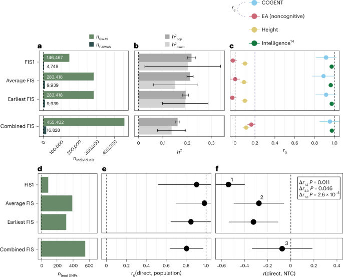
LDSC71 was used to compute genetic correlations and SNP heritabilities. This tool requires munged (parsed) sumstats. In munging, we aligned SNPs with those in the HapMap 3 (ref. 76) set using the ‘–merge-alleles’ flag. Heritabilities and genetic correlations were computed using the ‘–h2’ and ‘–rg’ flag, respectively, with default parameters. To estimate the genome-wide correlation between the direct effects and NTCs, we used the SNIPAR package correlate.py script33. We applied a block-jackknife procedure to test whether estimates differed significantly across imputation approaches. To do this, we derived the intersection of SNPs included in each GWAS, ordered them by chromosome and then by position, and divided them into 200 blocks of ~5,077 SNPs.
Identifying lead SNPs
The online platform for FUMA32 SNP2GENE was used to identify lead SNPs. First, independent significant SNPs are identified (P < 5 × 10⁻⁸, r2 < 0.6). Subsequently, identified significant SNPs are designated lead SNPs if they are independent from each other at a second threshold of r2 < 0.1.
Gene prioritization and tissue expression
MAGMA77 (as implemented in FUMA’s SNP2GENE process) was used for gene prioritization and tissue expression analyses using the results from the population-based GWAS. MAGMA aggregates SNP-level data into gene-level data and performs a gene-based association test to identify significantly associated genes. The gene window was kept at 0 kb, restricting analysis to SNPs located within a gene. Resulting gene-based P values were downloaded and FDR corrected using the Benjamini–Hochberg procedure. To obtain our set of prioritized genes, we selected protein-coding genes with an FDR < 1% that were also MANE select transcripts78. We then applied the SNP2GENE process in FUMA to test whether the significant genes were enriched in particular tissues; this takes the gene-level P values from MAGMA as input. We used expression data from 54 tissues from GTEx (v8; ref. 79) as reference data.
Within-family GWAS
We conducted within-family GWAS in UKB using the SNIPAR package33 in individuals with European ancestry. SNIPAR leverages the presence of genotyped first-degree relatives to impute missing parental genotypes, allowing for their downstream use to conduct within-family GWAS. We estimated pairwise kinship coefficients using KING80 and used default parameters to conduct the within-family GWAS using scripts provided in SNIPAR. We controlled for the same covariates as in the population GWAS. SNP heritability estimates were estimated using LDSC as described above. We filtered to SNPs with INFO score > 0.98 for all analyses using SNIPAR-imputed individuals, including the GWAS and PGI analyses.
Whole-exome sequencing data in UKB and quality control
Whole-exome-sequencing data were generated at the Regeneron Genetics Center, and the sequencing procedure has been described in previous studies. We used custom applets to perform quality control for the whole-exome sequencing data of 469,836 participants within the UKB research analysis platform. First, we used BCFtools norm to split and left-align multi-allelic variants in the population-level Variant Call Format files into separate alleles. Next, we performed genotype-level filtering using BCFtools filter separately for single nucleotide variants (SNVs) and insertions/deletions. Specifically, SNV genotypes with a depth below 7 and genotype quality below 20, or insertions/deletion genotypes with a depth below 10 and genotype quality below 20, were set to missing. We also applied a binomial test to check for an expected alternate allele contribution of 50% for heterozygous SNVs, and SNV genotypes with a binomial test P ≤ 0.0001 were set to missing. Finally, we recalculated the proportion of missing genotypes for each variant and excluded all variants with more than 50% missingness.
Next, we annotated the variants using the ENSEMBL Variant Effect Predictor (VEP; v104) with the –everything flag. For each variant, we prioritized a single ENSEMBL transcript based on whether the transcript was protein coding, MANE Select (v0.97) or the VEP canonical transcript. The variant consequence was prioritized based on severity as defined by VEP. After annotation, we grouped stop-gained, frameshift, splice acceptor and splice donor variants into a single PTV category. Missense and synonymous variant consequences were defined according to VEP criteria, and only autosomal variants within ENSEMBL protein-coding transcripts were retained for further analysis.
We further filtered variants by MAF, retaining only those with MAF <0.001%. These variants were annotated with LOFTEE, REVEL, AlphaMissense, and MPC for further filtering. For PTVs, only high-confidence PTVs defined by LOFTEE were retained. For missense variants, a damaging missense variant set was created by including variants with AlphaMissense scores > 0.56, REVEL scores > 0.5 and MPC scores > 2.
Exome-wide burden tests of rare coding variants
To examine the association between FIS and the burden of rare coding variants, we counted the number of rare PTVs, missense variants, damaging missense variants (as described above) and synonymous variants both in exome-wide and in high loss-of-function-intolerant (pLI > 0.9) genes. The variant burden was then used as the predictor variable in linear regression models, with FIS (observed, imputed and combined) as the response variables. The models were run in unrelated participants with European ancestry (n = 328,795). We controlled for the top 25 PCs, as well as age, sex, age2 and the interactions between age and sex, and age2 and sex72.
Gene-based burden test of rare coding variants
We performed gene-based burden tests on observed and combined FIS (standardized to mean 0 and variance 1) and EA (number of years of education) using a two-step regression analysis in REGENIE. As REGENIE accounts for relatedness and population structure, the gene-based tests were performed in all participants with European ancestry (n = 438,285; please note that this is lower than the sample size used for common-variant analyses, as not all participants had exome data). In the first step, REGENIE fits a stacked block ridge regression to produce a leave-one-chromosome-out genetic prediction of the focal phenotype. The association test is then carried out in the second step by fitting regression models conditioned on the leave-one-chromosome-out predictions. For both steps, we adjusted for sex, age, age2, sex-by-age interaction, sex-by-age2 interaction, the top 25 PCs and recruitment centers (as categorical variables) to control for population structure and age. The FIS scores were rank based and inverse-normal transformed, as recommended by REGENIE. EA was coded in ref. 81 by using individual reports of highest attained qualification, with ‘college or university degree’ counting as 20 years, ‘other professional qualifications’ as 15, ‘A levels/AS levels or equivalent’ as 13, ‘O levels/GCSEs or equivalent’, ‘CSEs or equivalent’ as 10 and ‘none of the above’ as 7. We ran both burden tests and SKAT-O tests on three consequence classes—PTV, damaging missense and PTV + damaging missense. Thus, for FIS we conducted 12 tests per gene (including 2 phenotypes, 2 statistical methods, 3 consequence classes). To account for multiple testing, we calculated the FDR using the Benjamini–Hochberg method across the vector of all P values and considered genes passing FDR < 1% as ‘significant’. For EA, we conducted six tests per gene as we only considered a single phenotype, and similarly accounted for multiple testing by calculating the FDR across a vector of all P values and considering genes passing FDR < 1% as ‘significant’. We used the DDG2P gene list downloaded on 5 February 2025 for annotating genes as ‘well-established’ developmental condition genes.
Replication analyses in external cohorts
Information about the replication cohorts (ALSPAC, MCS and INTERVAL) is given in Supplementary Methods. Quality control and imputation of genotype data in ALSPAC and MCS were conducted in ref. 82 and are summarized in Supplementary Methods, as is the preparation of the exome data, which was described in ref. 37. Quality control in INTERVAL was conducted in refs. 83,84 and is summarized in Supplementary Methods.
Cognitive performance measures
In ALSPAC, we considered IQ measured at age 8 using the Wechsler Intelligence Scale for Children test85. We included 5,283 unrelated children with genetically inferred European ancestry and at least one genotyped parent in our analyses. In MCS, we derived a cognitive performance measure as previously described in ref. 82 by fitting a one-factor model and calculating scores using ‘factanal’ and Bartlett scoring in R using the following measures: Bracken School Readiness at age 3 years, reading vocabulary at ages 3 and 5 years, pattern construction at ages 5 and 7 years, and word reading and progress in math at age 7 years. The summarized measure explained 39% of the variance, and we included a total of 5,621 unrelated children of genetically inferred European ancestry with at least one genotyped parent. In INTERVAL, participants completed an FI test identical in nature to the one completed by UKB participants in the first in-person wave at two time points 12 months apart (test–retest correlation = 0.65, P < 10−15). We took the average of the FIS for individuals who had two measurements. We included 20,328 unrelated individuals of genetically inferred European ancestry. All variables were standardized to have a mean of 0 and variance of 1.
Calculating PGIs
We used LDpred2-auto86 to calculate PGIs in ALSPAC, MCS and INTERVAL using the GWAS for observed FIS (that is, measured average FIS), combined FIS and combined FIS + COGENT GWAS meta-analysis. We also used unrelated individuals with European ancestries (Supplementary Methods) and generated LD reference panels restricted to HapMap 3 + SNPs86, which are designed to maximize genome-wide tagging coverage, improving performance across diverse ancestries compared to the original set. We used default parameters to calculate SNP weights for the PGIs. We then imputed missing parental genotypes in both cohorts (that is, if one but not both parents were genotyped) using SNIPAR33 as previously described82 and calculated PGIs with the SNP weights generated above using the pgs.py script. We filtered PGI SNPs to those with INFO score > 0.98 in each given cohort.
Estimating direct and population effects of PGIs on cognitive performance measures
To estimate the population effects of the PGIs, we standardized the PGIs as above and regressed the phenotypes on the individual’s PGI, 20 genetic PCs and sex, and additionally age and age2 in INTERVAL, using the ‘lm’ function in R. To estimate the direct effects in ALSPAC and MCS, we added the two parental PGIs and additional covariates to the previous regression. The coefficient estimated for the child’s PGI is the partial correlation between the PGI and the phenotype, and represents the direct genetic effect.
In MCS, we accounted for ascertainment biases due to the cohort’s nonrandom sampling scheme and attrition by incorporating sampling weights as previously described8. Briefly, we generated nonresponse weights using inverse probability weighting and multiplied these weights with the full UK sampling weights generated by the study. We then used these weights in the regression analyses conducted in MCS using the weights argument in the ‘lm’ function in R.
Multilevel mixed-effects regression
We used a multilevel mixed-effects regression to evaluate the association between discovery GWAS sample size and standardized PGI effect sizes using the ‘metafor’ package in R87. We regressed the PGI βs, weighted by their inverse variance to account for measurement error, on the logarithm of the GWAS discovery sample size.
Random intercepts were included for the cohorts (ALSPAC, MCS and INTERVAL) and for effect type (population and direct) nested within each cohort to account for heterogeneity in effect estimates across these groups. The model was specified as:
$${\beta }_{\left(\mathrm{ijk}\right)}={\gamma }_{0}+{\gamma }_{1}\mathrm{log}\left({n}_{\left(\mathrm{ijk}\right)}\right)+{u}_{{\rm{i}}}+{v}_{{\rm{j}}}\left(i\right)+{\varepsilon }_{\left(\mathrm{ijk}\right)}$$
where γ0 is the overall intercept, γ1 represents the fixed effect of log(n), uᵢ is the random effect for the ith cohort, vⱼ(i) is the random effect for effect type nested within the ith cohort and ε₍ᵢⱼₖ₎ is the residual error. We also ran the model using direct effects estimates alone, dropping the vⱼ(i) term.
Enrichment of de novo damaging variants in probands with neurodevelopmental conditions
We used previously published data from ref. 21 on three cohorts totaling over 31,000 exome-sequenced probands with developmental conditions and their parents to assess enrichment of damaging de novo mutations in the set of 12 genes with rare variant associations with FIS (FDR < 1%) that are not DDG2P genes.
We evaluated enrichment of de novo synonymous and nonsynonymous variants in the probands as follows. We used the null mutational model36 to compute, for each consequence class i, the cumulative per-site mutation rate μi,g across all callable variants of that class in a given gene g, that is, the summed mutation rate across all sites in a gene. The expected burden of de novo mutations of class i for a given gene-set G was then calculated as:
$${E}_{i,G}=\sum _{g\in G}{n}_{g}{\mu }_{i,g},$$
where ng is the total number of probands. We compared the observed count Oi of de novo mutations in class i to Ei by performing a one-sided Poisson test with rate parameter λ = Ei, calculating P(X ≥ Oi|X ~ Pois(λ)) as the significance of any excess de novo mutations. This framework allows assessment of whether damaging protein-truncating or missense variants occur more often than expected by chance, with synonymous variants serving as an internal negative control.
Replication of gene-based burden test results in ALSPAC and MCS
To replicate the results of our gene-based tests in UKB, we performed gene-set burden tests in ALSPAC and MCS. For both cohorts, we included only variants with a MAF lower than 0.1% in participants with European ancestry and had a gnomAD (v3; ref. 18) allele frequency of < 3 × 10⁻⁵ (corresponding to allele count < 5). As in UKB, we only retain high-confidence PTVs defined by LOFTEE18 and missense variants with an MPC score > 2. We then calculated the burden of PTVs for the following three gene sets: (1) all 26 genes discovered in UKB at FDR < 1%; (2) the FDR < 1% genes excluding the eight already identified in ref. 20; and (3) the 21 FDR < 1% genes that we only discovered when using combined FIS. We used linear regression models to examine the association between cognitive measures and the gene-set burden of PTVs in unrelated children with European ancestry in both the Avon Longitudinal Study of Parents and Children (ALSPAC; n = 5,283) and the MCS (n = 5,621), controlling for sex and population structure with the top ten PCs.
Reporting summary
Further information on research design is available in the Nature Portfolio Reporting Summary linked to this article.