
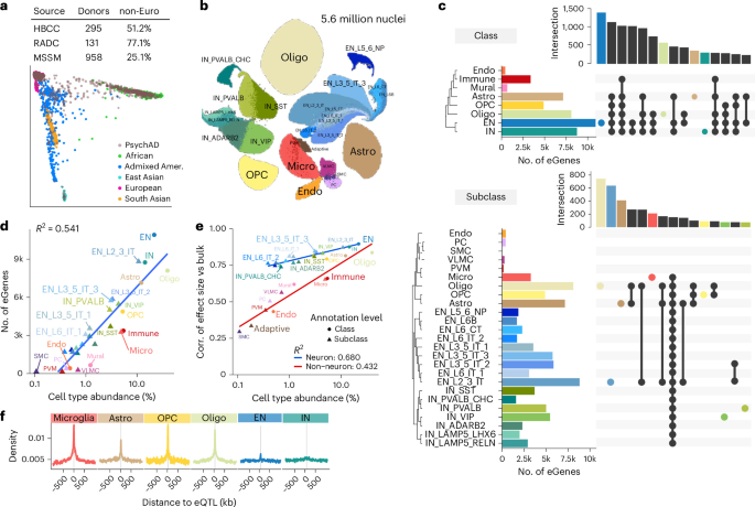
All procedures and research protocols were approved by the Institutional Review Board (IRBs) of Rush University Medical Center and the Mount Sinai and Mount Sinai/James J. Peters VA Medical Center. The autopsied brain specimens originated from brain donation programs at Rush University Medical Center/Rush Alzheimer’s Disease Center and the Mount Sinai Brain Bank, including samples collected from the James J. Peters VA Medical Center National Institutes of Health (NIH) Brain and Tissue Repository. All research conformed to the principles of the Declaration of Helsinki. Participants did not receive compensation. Sample numbers were determined by the availability of fresh brain autopsies. No statistical methods were used to predetermine sample size
Sample selection and preprocessing
Brain tissue from the DLPFC was obtained from 1,494 donors by the PsychAD Consortium24,25. The dataset comprised donors from three sources. The Rush Alzheimer’s Disease Center repository of tissue from the Religious Orders Study or Rush Memory and Aging Project46 provided 152 specimens; the Human Brain Collection Core provided 300; and the Mount Sinai Brain Bank (Mount Sinai School of Medicine) provided 1,042 specimens. The cohort includes similar numbers of males and females and spans the entire postnatal age range of 0 to 108 years. See previously published work24,25 for additional details about the donors and data processing.
Paired-end reads from snRNA-seq libraries were aligned to the hg38 reference genome using STAR solo47, and sample pools were demultiplexed through genotype matching with Vireo (v0.5.8)48. Following the generation of per-library count matrices, downstream processing was conducted using Pegasus (v.1.7.0)49 and scanpy (v.1.9.1)50.
We implemented a stringent quality control process to eliminate ambient RNA and preserve high-quality nuclei for further analysis. As part of our rigorous quality control pipeline, we initially tested for potential contamination using CellBender (v0.4.0)51, a deep generative model specifically designed to remove counts owing to ambient RNA molecules and random barcode swapping. In our initial assessment, however, we did not observe significant ambient RNA contamination across our datasets. In addition, to ensure the highest fidelity of the final processed object and to robustly confirm that our cell-type specificity results were not driven by background noise, we additionally performed an analysis using SoupX (1.6.2)52. This secondary validation confirmed that our data are free of significant ambient RNA effects.
Genomic DNA was extracted from frozen brain tissue using the QIAamp DNA Mini Kit (Qiagen), following the manufacturer’s instructions. The samples were genotyped using the Infinium Psych Chip Array (Illumina) at the Mount Sinai Sequencing Core. Pre-imputation processing involved running the quality control script HRC-1000G-check-bim.pl from the McCarthy Lab Group, using the Trans-Omics for Precision Medicine (TOPMed) program. Genotypes were phased and imputed on the TOPMed Imputation Server (https://imputation.biodatacatalyst.nhlbi.nih.gov). Samples were excluded if there was a mismatch between self-reported and genetically inferred sex, suspected sex chromosome aneuploidies, high relatedness (KING53 kinship coefficient of >0.177) or outlier heterozygosity (±3 s.d. from the mean). Additionally, samples with a sample-level missingness of >0.05 were excluded, as calculated within a subset of high-quality variants (variant-level missingness of ≤0.02). A total of 1,384 donors with genotype data and snRNA-seq data passing quality control were analyzed in this study.
Cell annotation
Cell annotations of the PsychAD dataset at the class and subclass level are provided in a companion paper24. Cellular taxonomy was defined using a divide-and-conquer strategy. From the full PsychAD dataset containing over six million nuclei, eight major cell classes were defined using the following steps: 6,000 highly variable genes (HVGs) were selected from mean and dispersion trends54 using default parameters (min_mean = 0.0125, max_mean = 3, min_disp = 0.5) and brain source as a batch variable after manually excluding sex and mitochondrial chromosomes. We used the k-nearest neighbor (kNN) graph calculated based on a harmony-corrected principal component analysis embedding space to cluster nuclei of the same cell type using the Leiden55 clustering algorithm. We used uniform manifold approximation and projection (UMAP)56 to visualize the resulting clusters. From the class-level clusters, we subsetted the data by each class. Re-calculating HVGs among cells in the same class allowed us to re-focus on a feature space that is more relevant for the same class of cells. A kNN graph was then calculated based on the harmony-corrected principal component analysis of the selected HVGs. Leiden clustering was used to annotate 27 subclass-level annotations. We iterated the same HVG–kNN–Leiden clustering for all 27 subclasses, yielding 67 subtypes of human brain cells. After obtaining annotations at three levels of hierarchy, the resulting clusters were aggregated into pseudobulk profiles, and cluster-wise Pearson correlation coefficients were calculated using existing human DLPFC57 and M1 (ref. 58) annotations. We matched the annotations based on both high correlation and specificity of the cell type.
Normalization of gene expression
Pseudobulk read counts were calculated by summing reads from the same individual using the dreamlet workflow59. As done in the companion paper24, we performed variance partitioning analysis to identify variables correlated with gene expression. This identified the proportion of mitochondrial expression as an important variable; it was regressed out to mitigate technical variability linked to batch effects, cell quality and potential stress-related artifacts. In addition, the effects of the sample pool and the influence of disease status were also controlled for by regression. Finally, the residuals were divided by the predicted standard deviation to produce Pearson residuals, excluding the impact of varying sequencing depths among the scRNA-seq libraries.
We applied the PEER package60 to detect hidden unobserved covariates. To find an optimal number of PEER factors to remove, we performed eQTL detection on the input expression matrix, normalized by pre-selected biological and technical covariates, varying the number of PEER factors from ten to 98 in increments of four. The setting with the most genome-wide significant eQTLs detected was used as the final result for downstream analysis (Supplementary Fig. 23).
Analysis of genetic regulatory variants at the pseudobulk level
Analysis was performed at the pseudobulk level. For each cell type, donors with at least five nuclei were retained in order to ensure stable donor-level expression estimates and to reduce noise from sparse sampling. Genes were filtered within each cell type to retain only those that were robustly expressed. This filtering procedure was implemented using edgeR::filterByExpr() and required that at least 40% of donors have a minimum count of five reads per gene. After quality control and filtering, the number of donors retained for each cohort varied (Supplementary Table 4).
The regression residuals used in the eQTL analysis were generated as follows. Expression for each cell type and each individual was computed as the log2 counts per million with a pseudocount of 0.25 after aggregating all corresponding nuclei. A precision-weighted regression model was fit for each expressed gene in each cell type with the dreamlet package (v1.4.1)59 using covariates for age, sex, postmortem interval, mitochondrial rate, ribosomal rate and disease status. From these models, Pearson residuals (that is, residuals divided by their standard errors) were computed for each expressed gene and cell type and used in downstream QTL analysis. Using the Pearson residuals identified 3.9–10.5% more genome-wide significant eGenes than using raw residuals (Supplementary Fig. 24).
In each cell class and subclass, eQTL analysis was performed for variants within 1 Mb of the transcription start site of each expressed gene. Imputed variants were filtered based on genotype completeness (95%), minor allele frequency (1%) and standard quality metrics (imputation INFO of >0.3) to ensure high-confidence association testing. Donors were required to pass quality control in both genotype and expression datasets. Given the diverse genetic ancestry of the individuals in this dataset, we used a linear mixed model to account for population structure and avoid false-positive findings resulting from genetic confounding61. We implemented this process using the mmQTL software (v1.5.0)7 to model a genetic relatedness matrix between all pairs of individuals as a random effect. Cis-eQTL analyses were performed exclusively on autosomal chromosomes. Variants and genes located on the X chromosome were excluded. Each cohort was analyzed separately, and eQTL results were combined using a fixed-effects meta-analysis.
Multiple-testing correction was performed using a two-step Benjamini–Hochberg FDR control framework, as done previously7. First, for each gene, all tested variants within the cis window were adjusted using the Benjamini–Hochberg procedure to control the FDR across variants tested for that gene. Second, we applied an across-gene correction by applying the Benjamini–Hochberg procedure across genes to control the genome-wide FDR.
Replication in independent cohorts
For the ROSMAP cohort of 424 donors and 1.5 million nuclei from the DLPFC, raw snRNA-seq counts were obtained from the Fujita22 dataset. Alignment, quality control, cell type annotation and eQTL analysis were performed as for the PsychAD data. The cell type composition is similar to the PsychAD cohort (Supplementary Fig. 22).
The Bryois dataset21 comprised three cohorts including 192 donors and 750,000 nuclei from the prefrontal cortex, temporal cortex and white matter across eight annotated cell types. They provided eQTL summary statistics that we used in our replication analysis.
Evaluating replication of genetic regulatory variants across datasets
We used the R package qvalue to estimate eQTL replication rates using Storey’s π1 statistic39. For a pair of datasets, we first extracted the most significant variant for genes with an eQTL in the discovery data. The P values from the replication dataset were then used to estimate Storey’s π1 value, which indicates the fraction of hypothesis tests for which the null is rejected. Thus, π1 is the estimated fraction of eQTLs that replicate in the second dataset. This metric of replication is useful because it does not depend on hard cutoffs for P values for FDR, and it has been widely adopted. The PsychAD cohort from the current study was used for discovery, and replication rates were evaluated using independent snRNA-seq data of human postmortem brain tissue from the Bryois21 and Fujita22 datasets.
Enrichment of OCRs around detected regulatory variants
To determine whether cell type-specific regulatory elements were enriched around eQTLs, we used the fdensity function in QTLtools (v1.3.1)62 to compute the number of functional elements that overlap each 10 kb bin in a 2 Mb window around the cis-eQTL. The OCR annotations were obtained from single-cell ATAC-seq data from human brain tissue26, and cell type-specific OCRs were defined as those found in only one cell type.
Fine-mapping of cis-eQTLs
We conducted fine-mapping with CAVIAR63 (v.2.0.0), which implements a probabilistic model to estimate posterior inclusion probabilities while accounting for local LD structure derived from study genotypes and assuming a single causal variant. We set the other parameters to their default values and output variants from 95% credible sets by ranking them by posterior inclusion probability until the cumulative posterior probability reached 0.95. We report the distribution of credible set sizes across loci, providing a quantitative summary of fine-mapping resolution.
Partitioning heritability based on statistical fine-mapping
S-LDSC was used to test whether custom variant annotations from statistical fine-mapping of eQTL signals were enriched for heritability attributable to genetic risk for complex traits3,64. Partitioned heritability analyses were conducted using only autosomal variants, consistent with standard S-LDSC analyses. For each eGene, statistical fine-mapping was used to compute a posterior inclusion probability for each cis-variant, retaining variants in the 95% credible set for each gene. Each variant in the genome is annotated with a probability value from this analysis. Variants not in a 95% credible set receive a value of zero, and variants evaluated for multiple genes receive the maximum probability value for the variant across these genes. This approach is termed ‘MaxCPP’ in a previous publication64. S-LDSC was then used to partition trait heritability using the constructed functional annotations, using the 1000 Genomes Phase 3 European ancestry reference panel. The estimated enrichment was used to measure the importance of each eQTL category to human complex traits or diseases. To rule out potential influences of correlation among eQTL categories, we aggregated the baselineLD model, which includes a set of 75 functional annotations from a previous publication65, to create functional annotations for the eQTL category, then ran S-LDSC jointly and assessed significance using the enrichment P value.
Proportion of disease heritability mediated by regulatory variants
Mediated expression score regression (MESC) estimates the proportion of disease heritability mediated by regulatory variants for a specific set of molecular traits27. We applied this approach to estimate the contribution of regulatory variants across cell classes and subclasses to the heritability of complex traits. MESC was then used to calculate mediated heritability with default settings. To estimate the joint contribution of subtypes from one cell class, we also ran meta-analyzed MESC using meta_analyze_weights.py. Following the package’s instructions, analysis was performed on all expressed genes. No additional filtering was performed based on cis-eQTL or trans-eQTL results, fine-mapping or other criteria.
Colocalization of genetic signals from regulatory and disease risk variants
To evaluate the relationship between molecular QTLs, we used the coloc R package to conduct colocalization analysis66. The summary results from meta-analysis were used as input for coloc. Colocalization was performed within overlapped regions between eQTL and GWAS summary statistics centered around the gene body. Consistent with previous work by our group8 and others67,68, no P value thresholds were used, so it is possible to identify colocalization with a locus that does not reach genome-wide significance. The phenotypic variance was set to 1 because we had normalized the summary results before meta-analysis; otherwise, parameters were set to their default values. We also applied an extension, moloc69, that applies this framework to identify the colocalization of three signals. For coloc analyses, we considered signals between two traits to be colocalized at a posterior probability of ≥0.8 (that is, PP4 ≥ 0.8).
Identifying shared and cell type-specific genetic regulatory effects
To determine how eQTL effects are shared between different cell types, we applied a multivariate Bayesian meta-analysis approach using the mashr software (v0.2.79)33. This software uses a Bayesian approach to shrink effect sizes across genes and cell types to estimate the posterior effect sizes and posterior probability that an effect has the correct sign. Following guidelines in the mashr documentation, we estimated the prior effect size distribution using a collection of genes expressed in all cell types and learned the empirical correlation structure using 600,000 randomly selected variant–trait pairings. For all genes with a genome-wide significant eQTL in at least one cell type, the variant with the smallest P value was selected, and the coefficient estimate and standard error were used in analysis with mashr. For genes not analyzed in a particular cell type owing to insufficient expression, values of zero were used for the coefficient, and 1 × 10⁶ was used for the standard error.
We extend this approach to develop a formal statistical test to identify cell type-specific genetic regulatory effects. Although the mashr analysis integrates results across cell types, the software characterizes the regulatory effect of a variant in one cell type at a time. Mashr tests whether a genetic effect is present in a given cell type. By contrast, we directly test whether a genetic effect is cell type-specific using a composite test that assesses whether the effect is non-zero in a given cell type while also being zero in all other cell types.
Here, we describe the math of the composite test. For a gene j and cell type i, mashr reports the local false sign rate defined as \({\text{lfsr}}_{j,i}=\min \left[p({\beta }_{i,j}\ge 0|\hat{\beta },\ldots ),p({\beta }_{i,\,j}\le 0|\hat{\beta },\ldots )\right]\), where \(({\beta }_{i,\,j}\ge 0|\hat{\beta },\ldots )\) is the probability that the true value of the regression coefficient is greater than zero given the estimated coefficient and other model parameters70. Thus, \({\text{lfsr}}_{i,\,j}\) is the posterior probability that the sign of the estimated coefficient does not agree with the sign of the true coefficient value, and it is more conservative than the local false discovery rate70. Then let \({p}_{i,\,j}=1-{\text{lfsr}}_{i,\,j}\) be the probability that the signs agree. For a given gene, this set of posterior probabilities can be used to estimate the probability of any combination of eQTL effects across cell types. Therefore, \({p}_{1,j}\) is taken as a conservative estimate of the probability that a genetic variant has a non-zero effect size in cell type 1, and \(1-{p}_{2,\,j}\) is taken as a conservative estimate that the effect is zero in cell type 2. Combining these estimates, the probability of a non-zero effect in cell type 1 and a zero effect in cell type 2 is \({p}_{1,j}\left(1-{p}_{2,j}\right)\), assuming the probabilities are independent. In general, the probability of an arrangement with non-zero effects in set 1 and all zero effects in set 2 is \(\left[{\varPi }_{i\in \text{set}1}{p}_{i,\,j}\right]\left[{\varPi }_{i\in \text{set}2}\left(1-{p}_{i,\,j}\right)\right]\).
Owing to limited statistical power to detect eQTLs in high-resolution cell types, it is often too restrictive to ask, for example, whether an eQTL effect is non-zero in all excitatory neuron subtypes. Instead, we can ask whether there is a non-zero effect in at least one subtype by evaluating \(1-\left[{\varPi }_{i\in \text{set}1}\left(1-{p}_{i,\,j}\right)\right]\).
Aging-related dynamic eQTL detection
As part of the PsychAD Consortium, an analysis of the transcriptional dynamics of normal aging across the human lifespan was performed in a companion paper34. Using the PsychAD dataset, the authors extracted data from 284 neurotypical postmortem donors aged 0–97 years, comprising 1.3 million nuclei, and divided donors into six developmental groups: neonatal (0–1 year old, n = 9), childhood (2–11 years, n = 11), adolescence (12–19 years, n = 33) and young (20–39 years, n = 54), middle (40–59 years, n = 95) and late adulthood (≥60 years, n = 82). The authors34 then constructed a pseudotime trajectory within each cell type, using a supervised method incorporating donor age by applying the UMAP of MATuration (UMAT) method. This approach constrains the projection to a low-dimensional space by restricting UMAP neighbor selection to nuclei from adjacent developmental stages35. This constraint produces a pseudotime trajectory that is consistent with the known developmental ordering of the donors based on age. Nuclei from the full PsychAD dataset were then projected onto this UMAT space, and each nucleus was assigned a pseudotime score corresponding to its cell type.
Dynamic QTL analysis was then performed at the single-nucleus level for each cell type by testing whether the estimated genetic effect of a given variant on a gene expression trait changed along the pseudotime trajectory. For a given cell type, every nucleus was included in a regression model that tested an interaction effect between genetic variant and pseudotime. Raw count data for gene expression were analyzed using a negative binomial mixed model (NBMM), with donor as a random effect. We found this NBMM to be critical to controlling the false-positive rate in our dataset. Covariates for library size, age, sex and mitochondrial rate were included as fixed effects. Analyses were implemented using the glmer.nb() function in the lme4 R package71:
glmer.nb(y~pseudotime+SNP+pseudotime*SNP+covariates,…)
and P values were computed from a Wald test.
NBMM analysis at the single-nucleus level is very demanding, requiring approximately 1 h of processing time per regression because of the large number of nuclei included in each analysis (astrocytes, 763,000; excitatory neurons, 1.45 million; immune cells, 331,000; inhibitory neurons, 973,000; oligodendrocytes, 2.28 million; and OPCs, 363,000). Yet we found this NBMM to be critical to controlling the false-positive rate in our dataset. Owing to the high computational time, we followed the approach of previous work13,23 and analyzed one variant per gene for each cell type, selecting the top variant from the standard pseudobulk cis-eQTL analysis for each cell type.
The enrichment of genes with dynamic regulatory signals for colocalization with disease traits was evaluated as follows. For a cell class i with \({d}_{i}\) dynamic eGenes, the number of genes that also have a colocalization signal was computed. The null distribution of this count was evaluated by randomly sampling \({d}_{i}\) genes and evaluating the overlap with genes with a colocalization signal. The standard error of the overlap for each cell type was evaluated using 100 rounds of random sampling.
Trans-eQTL detection
Performing trans-eQTL analysis on a large number of single-nucleotide polymorphisms (SNPs) is computationally expensive and incurs a substantial multiple-testing burden. Following previous work13, we addressed both of these issues by selecting lead variants, including 56,204 eSNPs from the cis-eQTL analysis and 45,088 genome-wide significant variants from eight brain disease GWAS studies (that is, variants with P < 5 × 10⁻⁸ in AD, binge eating disorder, bipolar disorder, MDD, Parkinson’s disease, SCZ, attention deficit–hyperactivity disorder and autism spectrum disorder). Analysis was performed across all expressed genes in each cell class and restricted to autosomes, and excluded the X chromosome because of the increased statistical and biological complexity associated with modeling long-range regulatory effects involving sex chromosomes, yielding 8.74 billion tests. SNP genotype was included as the dependent variable in all gene–variant pairings in the linear regression model we tested. We defined trans-variants as variants located more than 5 Mb from target genes, and focused on autosomal chromosomes, excluding any signal within major histocompatibility complex regions. Genes with a mappability score of <0.8 were excluded to avoid false-positive trans-eQTL findings caused by reads mapping to multiple locations in the genome10,72.
We applied multiple-testing corrections at two levels following the approach of widely used methods for cis-eQTL analysis62,73. For a given gene, the lead eQTL variant is defined as the variant with the smallest P value from all variants tested for that gene. Other software programs use permutation analysis to compute gene-level P values that correct for this multiple testing62,73. Instead of performing computationally expensive permutations, we applied a Šidák correction to report a gene-level P value corrected for testing k variants, using \(k=1\times {10}^{5}\). Letting \({P}_{\min }\) be the smallest P value observed for a given gene, the Šidák-corrected P value for the gene is \({P}_{S{idak}}=1-{\left(1-{P}_{\min }\right)}^{k}\). Given that we performed trans-eQTL analysis for six cell classes, gene-level P values were computed for each cell class. A second round of multiple-testing correction was applied across all genes and cell types by using the Benjamini–Hochberg method74 on these gene-level P values. Study-wide significant trans-eQTLs were identified at an FDR of 5%.
Mediation analysis of cis-mediated trans-eQTLs
To identify trans-eQTLs with evidence of mediation, we limited our exploration to trans-eSNPs with high LD (r2 ≥ 0.75) with at least one peak eQTL variant within 1 Mb. We applied the strategy developed in a previous publication75 to calculate the indirect impact of trans-SNPs on trans-eGenes. Multiple-testing correction using the Benjamini–Hochberg approach was applied to control the study-wide FDR at 5%.
Analysis of the X chromosome
We performed analysis on the X chromosome at the class and subclass level following the approach used by GTEx76. For variants located in the non-pseudoautosomal regions of the X chromosome, we accounted for sex-specific genotype dosage. Given that males are hemizygous for the X chromosome, their genotypes were coded as 0 (hemizygous reference) or 2 (hemizygous alternative), effectively doubling the allele dosage to match the diploid scale used for females. Genotypes in females were treated the same as autosomal variants (0, 1 or 2). For variants located in the pseudoautosomal regions of the X chromosome, genotypes were treated as autosomal because these regions are present on both the X and Y chromosomes and behave as diploid in both sexes. We then applied the same analysis pipeline as for autosomal chromosomes to run eQTL detection. Analysis was performed on each brain bank separately, and the results were combined using a fixed-effect meta-analysis. Effect size estimates showed high concordance across cell types, with sign concordance rates ranging from 84.8% to 97.8% (Supplementary Fig. 26). This analysis revealed between eight and 301 eGenes at the class level and between one and 213 eGenes at the subclass level (Supplementary Fig. 27).
Reporting summary
Further information on research design is available in the Nature Portfolio Reporting Summary linked to this article.