Nucleotide dependency analysis of genomic language models detects functional elements

SpeciesLM training

For SpeciesLM metazoa, we obtained metazoan genomes comprising 494 different species from the Ensembl 110 database36. For each annotated protein-coding gene, we extracted 2,000 bases 5′ to the start codon and trained a species-aware masked language model on this region. We followed the training and tokenization procedure outlined in Species-aware gLMs4, but kept the batch size at 2,304, despite increasing the input sequence length, resulting in approximately twice as many tokens seen during training as in SpeciesLM fungi 5′. We used rotary positional encoding to inject positional information into the Transformer blocks.

For SpeciesLM fungi, we deviated from the above recipe by tokenizing each base of the sequences discussed in ref. 4 separately (single nucleotide, 1-mer tokenization) and using learned absolute positional encodings. To stabilize training, we increased dropout in the multilayer perceptron layers of the transformer to 0.2 and set it to 0.1 for attention dropout.

Overall, we improved the training efficiency by fusing biases of the linear layers, the multilayer perceptron in the transformer and the optimizer using Nvidia Apex. We used FlashAttention2 (ref. 51) to train all models.

Nucleotide dependencies and variant influence score

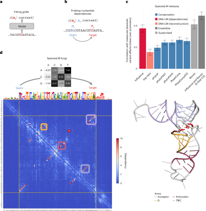
We define the dependency between a variant nucleotide kalt at position i and a target position j as

$${e}_{i,j,{k}_{\mathrm{alt}}}=\max {\left\{\left|{\log }_{2}\left(\frac{{\rm{o}}\hat{{\rm{d}}}\mathrm{ds}\left({n}_{\!j}={k|}{n}_{1},\ldots ,{n}_{i}={k}_{\mathrm{alt}},\ldots ,{n}_{N}\right)}{{\rm{o}}\hat{{\rm{d}}}\mathrm{ds}\left({n}_{\!j}={k|}{n}_{1},\ldots ,{n}_{i}={k}_{\mathrm{ref}},\ldots ,{n}_{N}\right)}\right)\right|\right\}}_{k{\rm{\in }}\left\{{\rm{A}},{\rm{C}},{\rm{G}},{\rm{T}}\right\}}$$

where k is one of the four possible nucleotides A, C, G or T; ni and nj are the nucleotides at position i and j, respectively; kref is the nucleotide in the reference, nonaltered input sequence, and kalt is the nucleotide in the alternative sequence. The odds estimates are computed from the predictions of a gLM under consideration. For this computation, none of the nucleotides (including the target nucleotide) is masked.

The variant influence score \({{e}_{i,k}}_{\mathrm{alt}}\), for a sequence of N nucleotides, is defined by averaging the dependencies on a variant nucleotide at position i across all positions j = 1, …, N such that \(j\ne i\).

A nucleotide dependency ei,j between a query position i and a target position j on a sequence of N nucleotides is given by:

$${e}_{i,j}=\max {\left\{\left|{\log }_{2}\left(\frac{{\rm{o}}\hat{{\rm{d}}}\mathrm{ds}\left({n}_{\!j}={k|}{n}_{1},\ldots ,{n}_{i}{\rm{\ne }}{k}_{\mathrm{ref}},\ldots ,{n}_{N}\right)}{{\rm{o}}\hat{{\rm{d}}}\mathrm{ds}\left({n}_{\!j}={k|}{n}_{1},\ldots ,{n}_{i}={k}_{\mathrm{ref}},\ldots ,{n}_{N}\right)}\right)\right|\right\}}_{k{\rm{\in }}\left\{{\rm{A}},{\rm{C}},{\rm{G}},{\rm{T}}\right\}}$$

We compute dependencies for all i,j pairs such that \(i\ne j,\) that is we do not consider self-dependencies.

In autoregressive models, a query variant cannot directly affect the prediction of a target position located 5′ of the query. Thus, to obtain the lower triangular matrix of the dependency map, we also run the model on the reverse strand.

In the SpeciesLM metazoa, which predicts nucleotides as overlapping 6-mers, the procedure needs to be adapted to yield one prediction for each target nucleotide. This is achieved by first computing for each of the six 6-mers that overlap the target nucleotide of interest, which probability it implies for this target nucleotide, as previously described4. We then average these six probabilities to obtain a single probability.

For the Nucleotide Transformer models, which predict only nonoverlapping 6-mers, we use a similar approach. Consider the case of predicting the probability of observing nucleotide n at position i of the sequence. In the tokenized sequence, this nucleotide has position p in the kth 6-mer where:

$$k=\left\lfloor \frac{i}{6}\right\rfloor$$

$$\begin{array}{cc}p=i & \mathrm{mod}6\end{array}$$

The model predicts a distribution over all 46 possible 6-mers at position k. We first discard all predictions corresponding to 6-mers that contain a nucleotide that differs from the reference sequence at any location other than p—which leaves only four 6-mers. We renormalize so that the predicted probability of these remaining 6-mers sums to one. We then record the (renormalized) probability of the 6-mer that has the desired nucleotide n at position p.

Apart from extracting nucleotide-level probabilities with the above-mentioned method, we have also experimented with computing the probability for a nucleotide at position i as the sum of all k-mers containing that nucleotide at that position. Evaluation of nucleotide dependencies within tRNAs revealed a worse performance with this method.

Variant impact benchmarks

As our metric of variant impact, we used the variant influence score. This average is computed over the full receptive field of the model for the SpeciesLM. For Nucleotide Transformer models, we only average over the central 2 kb, so as to facilitate comparisons. Nevertheless, we provide the full sequence context for which this model has been trained.

For comparison, we also calculated a variant effect score based on the gLM reconstruction at the query variant. Specifically, this score is the log ratio between the predicted probability of the variant nucleotide and the predicted probability of the reference nucleotide5,6.

Finally, we downloaded conservation scores (PhyloP and PhastCons) for human and S. cerevisiae from the University of California, Santa Cruz genome browser database21,22,23,24,52. For humans, these include the conservation scores based on the 100-way, 447-way and 470-way alignment.

Promoter saturation mutagenesis

Promoter saturation mutagenesis (ref. 20) data mapped to hg38 were provided by V. Agarwal (mRNA Center of Excellence, Sanofi, Waltham, MA, USA). As discussed in ref. 29, we excluded the FOXE1 promoter due to the low replicability of the measurements, leaving nine promoters and comprising 8,635 variants. Variants were then intersected with the human gene 5′ regions (that is, the regions 2-kb 5′ of annotated start codons). Then, the variant influence score was calculated for each variant measured in the assay from the LM dependencies for these regions. The variant influence score was then correlated with the absolute value of the measured log2 fold change in expression. This correlation was computed for each promoter and then averaged across promoters.

To determine confidence intervals, we performed 100 bootstrap samples per promoter and recomputed the correlation for each bootstrap sample. The confidence interval was defined by adding/subtracting two standard deviations of the average correlation.

eQTL variants

For human eQTL, we downloaded SUSIE26 fine-mapped GTEx eQTL data from EBI. We then intersected these data with the human gene 5′ regions. This procedure, by design, enriches for promoter eQTL. Similar to the details in ref. 29, we considered every eQTL variant with a posterior inclusion probability higher than 0.9 as putative causal and we considered any eQTL variant with posterior inclusion probability lower than 0.01 as putative noncausal. We only considered putative noncausal eQTL intersecting regions, which also include at least one causal eQTL. This procedure gave 2,958 eQTL variants, of which 1,631 were classified as putative causal. Then, the influence score for each variant was computed based on the nucleotide dependencies in these regions. We ranked variants according to the influence score. Confidence intervals were computed using bootstrapping as before.

For yeast eQTL, we downloaded the results of an MPRA study assessing candidate cis-eQTL variants27. After this study, we classify any eQTL variant with false discovery rate < 0.05 in the MPRA assay as causal and we classify any eQTL with (unadjusted) P value of >0.2 as noncausal. This yielded 3,056 eQTL variants, of which 379 were classified as causal. These eQTL variants were then intersected with yeast gene 5′ regions and influence scores were computed from the SpeciesLM fungi dependency maps. Confidence intervals were computed using bootstrapping as before.

Clinvar

We used ClinVar version 2023_07_17 (ref. 19), previously downloaded from https://ftp.ncbi.nlm.nih.gov/pub/clinvar/vcf_GRCh38/. We considered noncoding any variant in the categories ‘intron_variant’, ‘5_prime_UTR_variant’, ‘splice_acceptor_variant’, ‘splice_donor_variant’, ‘3_prime_UTR_variant’, ‘non_coding_transcript_variant’, ‘genic_upstream_transcript_variant’ and ‘genic_downstream_transcript_variant’. As discussed in ref. 53, we considered as pathogenic any variant classified as pathogenic or likely pathogenic and as benign any variant classified as benign or likely benign. We excluded variants with fewer than one review star. This resulted in 385,572 variants, of which 22,313 were classified as pathogenic.

As most ClinVar variants fall outside the 5′ regions of genes, we chose not to intersect with these regions. Instead, we computed the dependency map centered on the variant of interest. Confidence intervals were computed using bootstrapping as before.

Borzoi

We ran Borzoi in mixed precision to reduce computational overhead using the PyTorch Borzoi package. Replicate zero of Borzoi was used for all analyses. For the eQTL analysis, we computed the L2 score as discussed in ref. 25. We used the tissues of borzoi predictions matching the eQTLs. If several Borzoi tracks matched the tissue, we averaged the scores across these tracks. For ClinVar, we followed a similar approach, except that we collected Borzoi predictions for all tissues and assays. We then computed the L2 score across tracks to give a tissue-agnostic and mechanism-agnostic variant-effect score.

For the Kircher saturation mutagenesis dataset, we computed the logSED score as discussed in ref. 25. We mapped the cell types used in the assay to Borzoi tracks as follows: for the GP1BB, HBB, NHBG1 and PKLR promoters, we used ‘RNA:K562’; for the F9 and LDLR promoters, we used ‘RNA:HepG2’; for HNF4A and MSMB, we used ‘RNA:kidney’ (as HEK293 is originally a kidney cell) and for TERT, we used ‘RNA:astrocyte’ (as glioblastoma are cancerous astrocytes).

Integrative model using Borzoi and the influence score

We integrated Borzoi and the influence score using logistic regression—for the eQTL and ClinVar predicitions—and using linear regression for the mutagenesis data using fivefold cross-validation scheme for all benchmarks. Notably, for the Kircher saturation mutagenesis task, model fitting and cross-validation were performed separately for each promoter, and performance was then averaged across folds and promoters.

Alternative dependency metrics

All benchmarks on alternative dependency metrics were performed on the SpeciesLM fungi.

Gradient-based

We computed the gradient of the prediction for each nucleotide at position i with respect to each nucleotide at position j yielding a 4 × 4 matrix. To achieve this, we first replaced the tokenization layer with a one-hot encoding and a linear layer, which map the one-hot encoded nucleotides to their respective token embeddings. We then propagated gradients from each target nucleotide prediction to each one-hot encoded input nucleotide. As a metric of nucleotide dependency, we then used the maximum absolute value across the 4 × 4 matrix of each i,j position.

Mask-based

Masked-based dependencies are computed as:

$${e}_{i,j}=\max {\left\{\left|{\log }_{2}\left(\frac{{\rm{o}}\hat{{\rm{d}}}\mathrm{ds}\left({n}_{\!j}={k|}{n}_{1},\ldots ,{n}_{i}=\left[\mathrm{MASK}\right],\ldots ,{n}_{N}\right)}{{\rm{o}}\hat{{\rm{d}}}\mathrm{ds}\left({n}_{\!j}={k|}{n}_{1},\ldots ,{n}_{i}={k}_{\mathrm{ref}},\ldots ,{n}_{N}\right)}\right)\right|\right\}}_{k{\rm{\in }}\left\{{\rm{A}},{\rm{C}},{\rm{G}},{\rm{T}}\right\}}$$

where ‘[MASK]’ stands for the mask token, k belongs to one of the four possible nucleotides A, C, G or T; ni and nj are the nucleotides at position i and j, respectively; kref is the nucleotide in the reference, nonaltered input sequence.

S. cerevisiae tRNA structure benchmark

S. cerevisiae genome assembly version R64-1-1 and annotation version R64-1-1.53 were downloaded from EnsemblFungi36. The S. cerevisiae tRNA secondary structures were downloaded from GtRNAdb54. We considered only the tRNAs overlapping the 1 kb 5′ regions to any yeast start codon, yielding 172 tRNA sequences. Subsequently, dependency maps on tRNAs were processed by taking the maximum between ei,j and ej,i. This symmetrizes the dependency map and achieves one unique score per pair of positions in the tRNA sequence. We then used this score to predict whether a pair of nucleotides belonged to a secondary structure contact.

Assessment of donor–acceptor dependencies in S. cerevisiae

We extracted intron sequences by selecting the regions within annotated gene intervals that lie between exon annotations. This resulted in 380 sequences. We then retained only introns bounded by canonical splice site dinucleotides GT and AG, yielding 272 sequences. We then computed the average dependency between every donor and acceptor nucleotide within the intron as a measure of dependency between the donor and acceptor sites. We designed two negative sets for a given intron. For the negative set ‘Decoy acceptor’, we compute the average dependency between donor nucleotides and each AG dinucleotide within the intron that does not include the acceptor site. For the negative set ‘Matched distance’, we sampled four random dependencies between nucleotides that were as distant from each other as the donor was from the acceptor, without including the donor or acceptor themselves.

TF motif mapping

We downloaded FIMO PWM scan results from http://www.yeastss.org (ref. 55) and Chip-Exo TF binding peaks from http://www.yeastepigenome.org (ref. 31). We then extracted all Chip-Exo peaks for the available PWMs. We excluded PWM matches for which no Chip-Exo data were available for the corresponding factor. This procedure yielded data for 68 TFs. We annotated every nucleotide within 1 kb 5′ of a start codon as part of a binding TF motif if it is (1) part of a PWM match with P value of <0.01 and (2) this PWM match is within ten bases of a Chip-Exo peak of the corresponding TF. We defined the positive class in this way to ensure that we capture nucleotides relevant for determining binding (that is, motif) rather than all nucleotides close to a Chip-Exo peak, regardless of their role in binding. This resulted in 92,117 binding nucleotides out of a total of 6,538,427. We designated a nucleotide as repeat if it was masked by RepeatMasker. We extracted this information from the soft-masked GTF provided by Ensembl36.

The 69-way alignment

We used progressive cactus56 to align 69 budding yeast species using default parameters and specifying S. cerevisiae as reference quality genome. We then extracted fourfold degenerate sites and used phyloFit with the EM algorithm to estimate a neutral model. Using this neutral model and the alignment, we ran phastCons with the parameters –rho 0.3 –estimate-rho –target-coverage 0.4 –expected-length 23, which correspond to the parameters used in the seven-way alignment21. We also ran phyloP22, with –method LRT –mode CONACC.

Dependencies in rare-variant-associated aberrant splicing

We computed dependency maps for all rare SNVs associated with splicing outliers in GTEx28 as described earlier32. Because the input length of SpliceBert14 is limited to 1,024 bp, the complete set of variant outlier pairs (n = 18,371) was filtered such that the variant and associated outlier junction were located within an 800-bp window (n = 1,811) and 100 bp of sequence was added from the maximum and minimum positions of the variant and outlier junction splice sites. For each variant location, we extracted the average value of the dependency map at the intersection of either variant and outlier donor dinucleotide or variant and outlier acceptor dinucleotide. This variant effect score was compared against a background score. This background score was computed as the mean over all dependencies that were as distant from each other as the variant was from the outlier donor (matched distance) or the outlier acceptor. The scores were filtered for a minimum distance of 5 bp between the variant and splicing dinucleotide to filter values near the diagonal corresponding to self-interactions. Variant categories were annotated with the Ensembl variant effect predictor (VEP)57. For each variant, the most severe VEP annotation was considered. For the ‘exon’ category, the following VEP categories were grouped together: synonymous_variant, missense_variant, stop_lost, stop_gained.

Genome-wide search for parallel and antiparallel dependencies

We scanned dependency maps for parallel and antiparallel dependencies using 5 × 5 convolutional filters. We constructed the antiparallel filter by populating the antidiagonal of a zero-filled 5 × 5 matrix with ones, and for the parallel filter, by populating the diagonal with ones. We then centered each filter by subtracting the mean value from each position to ensure that a convolution on a uniform 5 × 5 region yields a result of zero. We applied these filters to dependency maps from SpeciesLM fungi (both filters) and RiNALMo (antiparallel filter only)4,7.

Search for parallel and antiparallel dependencies in fungi using the SpeciesLM fungi

For the SpeciesLM fungi, we have computed dependency maps spanning 1 kb 5′ of each annotated start codon on a set of representative fungi species, including Agaricus bisporus, Candida albicans, Debaryomyces hansenii, Kluyveromyces lactis, Neurospora crassa, S. cerevisiae, S. pombe and Yarrowia lipolytica. The genomes and annotation files for each species were downloaded from EnsemblFungi release 53 with accessions GCA_000300555.1, GCA000182965v3, GCA_000006445.2, GCA000002515.1, GCA_000182925.2, GCA_003046715.1, GCA_000002945.2 and GCA_000002525.1, respectively.

All regions annotated as ‘five_prime_utr’, ‘three_prime_utr’, ‘intron’, ‘CDS’, ‘pseudogene_with_CDS’ and other regions (for example, nonannotated introns) inside an annotated gene interval were categorized as protein-coding gene. All regions annotated as ‘tRNA’, ‘tRNA_pseudogene’, ‘rRNA’, ‘snRNA’, ‘ribozyme’, ‘SRP_RNA’, ‘snoRNA’, ‘RNase_P_RNA’ and ‘RNase_MRP_RNA’ were categorized as structured RNA. Finally, all regions annotated as ‘transposable_element’, ‘pseudogene’ and regions without any annotation were considered as intergenic.

Search for antiparallel dependencies and RNA structure in E. coli using RiNALMo

For RiNALMo, we computed dependency maps for regions 100, 200 and 500 bp before each annotated start codon in E. coli str. K-12 substr. MG1655, whose genome and annotation were downloaded from GenBank58 with accession U00096.3.

As candidates for a new RNA structure, we first filtered positions whose convolution value is greater or equal to 25 to select only high-value antiparallel dependencies, resulting in a filtered convolved dependency map. Next, we counted the unique number of antidiagonals potentially belonging to one stem by extracting the unique i + j nonzero positions supported by at least three nonzero values.

As candidates for a new structure, we selected maps suggesting the existence of at least two potential stems.

RNA secondary structure benchmarking

We downloaded the database of secondary structures Archive II37, which includes 3,865 curated RNA structures across nine families (5S rRNA, SRP RNA, tRNA, tmRNA, RNase P RNA, group I intron, 16S rRNA, telomerase RNA and 23S rRNA). For each structure, we generated the dependency map with the pretrained RiNALMo and retained the largest of the two dependency map entries for each pair of nucleotides (maximum of i,j and j,i). The AUROC curve was computed for each structure against the Archive II secondary structure annotations.

Benchmarking of canonical and noncanonical RNA contacts

We downloaded the database of RNA structures CompaRNA38, which is a compilation of RNA contacts based on 201 available RNA structures in the Protein Data Bank by RNAView59. Contacts are classified either as ‘standard’ or as ‘extended’. While the first includes only canonical AU, GC and wobble GU pairs in the cis-Watson–Crick/Watson–Crick conformation60, the latter calls all interacting bases regardless of their conformation, including noncanonical or tertiary contacts. Of the 201 structures, 196 had a length below the maximum input length of RiNALMo (1,022 nt). For each structure, we generated the dependency map using the pretrained RiNALMo and retained the largest entry from the two dependency maps for each pair of nucleotides. Similarly, the same structures were also evaluated with the fine-tuned RiNALMo model version rinalmo_giga_ss_bprna_ft, resulting in a predicted value for each pair of nucleotides. To evaluate their performance in predicting noncanonical contacts, we excluded all canonical contacts and computed the AUROC curve for all remaining positions across all structures. Significance between ROC AUCs was determined by bootstrapping over 10,000 permutations.

Comparison with RNAalifold

We evaluated the performance of the dependency maps against RNAalifold61, a standard alignment-based method for predicting a consensus RNA structure by incorporating sequence covariation from a set of aligned RNA sequences as input. For this, we use the 201 PDB entries in CompaRNA that had at least one Rfam match and consider two subsets. The first subset consisted of the 33 PDB sequences that contained an exact sequence match between the PDB entry and at least one Rfam seed alignment. In case of multiple matching Rfam seed alignments (for example, ribosomal RNA), we considered an arbitrarily chosen single Rfam seed alignment to avoid confounding the evaluations by duplicates. The second subset consisted of the remaining 168 sequences. For this, we used nhmmer (v3.1b2)62 to find homologous sequences within a database of 220,478 bacterial and archaeal genomes and plasmids downloaded from NCBI. After removing sequences longer than 1,022 nt (the maximum context length for which the gLM RiNALMo has been trained), this resulted in 67 sequences with hits in the database.

On the first subset, we use the Rfam seed alignments as input to RNAalifold. To assess the robustness of the analyses to the alignment procedure, we additionally realigned the sequences in the seed alignments using Clustal-Omega (v1.2.4)63 and MAFFT (v7.525)64. For the second subset, we performed sequence alignments using both Clustal-Omega and MAFFT, limiting the alignments to a maximum of 1,000 sequences (by aligning the PDB sequence to the top 999 nhmmer hits) to reduce computation time. On both subsets and from each alignment, a base-pair probability matrix corresponding to the predicted RNA structure was generated using RNAalifold available through the ViennaRNA (v2.6.4) package65. RNAalifold was run in the following two modes: using the default energy model (command: RNAalifold -p) and with RIBOSUM scoring (command: RNAalifold -p -r).

Pseudoknot benchmark

We downloaded the compendium dataset bpRNA-1m(90) that contains 28,370 annotated RNA structures with less than 90% sequence similarity obtained from the databases CRW, tmRNA, SRP, tRNAdb2009, RNP, RFAM and PDB39. From these, we extracted all structures that contain pseudoknot contacts and are no longer than 1,022 nt (the maximum context length for which the gLM RiNALMo has been trained). These resulted in 2,530 structures of varying lengths and sources. We then extracted the pseudoknot contacts from the dot-bracket notation provided by bpRNA that takes into account non-nested pairs39. Finally, we computed the dependency maps for each one of these structures and evaluated their ability to predict whether a pair of nucleotides belongs to a pseudoknot contact (positive set) or does not belong to a structure contact (pseudoknot or canonical structure contact—negative set).

DMS-MaPseq analysis of E. coli cells

E. coli TOP10 cells were grown in LB broth at 37 °C with shaking until OD600 = 0.5, after which dimethyl sulfate (DMS; Sigma-Aldrich, D186309), prediluted 1:4 in ethanol, was added to a final concentration of 200 mM. Bacteria were incubated for 2 min at 37 °C, and reaction was quenched by addition of 0.5 M final DTT. Bacteria were pelleted by centrifugation at 17,000g for 1 min at 4 °C, after which they were resuspended in cell pellets in 12.5-μl resuspension buffer (20 mM Tris–HCl pH 8.0; 80 mM NaCl; 10 mM EDTA pH 8.0), supplemented with 100 μg ml−1 final lysozyme (L6876, Merck) and 20 U SUPERase·In RNase Inhibitor (Thermo Fisher Scientific, A2696), by vortexing. After 1 min, 12.5-μl lysis buffer (0.5% Tween-20; 0.4% sodium deoxycholate; 2 M NaCl; 10 mM EDTA) were added, and samples were incubated at room temperature for 2 additional min. Then 1 ml TRIzol Reagent (Thermo Fisher Scientific, 15596018) was added, and RNA extracted as per the manufacturer’s instructions. rRNA depletion was performed on 1 μg total RNA using the RiboCop for Bacteria kit (Lexogen, 126). DMS-MaPseq library preparation was performed as previously described41. After sequencing, reads were aligned to the E. coli str. K-12 substr. MG1655 genome (GenBank, U00096.3), using the rf-map module of the RNA framework66 and Bowtie2 (ref. 67). Count of DMS-induced mutations and coverage and reactivity normalization were performed using the rf-count-genome and rf-norm modules of the RNA framework. Experimentally informed structure modeling was performed using the rf-fold module of the RNA framework and ViennaRNA (v2.5.1)67.

RNA structure covariation analysis

Covariation analysis was performed using the cm-builder pipeline (https://github.com/dincarnato/labtools) and a nonredundant database of 7,598 representative archaeal and bacterial genomes (and associated plasmids, when present) from RefSeq68.

Evaluation of artificial forward and inverted duplications

We generated random sequences of 100 nucleotides by sampling from regions 1 kb 5′ of the start codon in S. cerevisiae to ensure a representative GC content and shuffling the sequences to destroy potential functional elements. Additionally, we created 100 unique duplicated sequences, ranging from 2 to 20 nucleotides in length, by randomly sampling each nucleotide with equal probability. Each duplicated sequence was then inserted into a uniquely generated 100-nucleotide sequence at a random distance from each other, ensuring no overlaps occurred. We used the SpeciesLM fungi to generate dependency maps for each sequence. We then computed average dependencies by taking the mean of the dependencies between nucleotides and their duplicates. This involved averaging across a parallel diagonal for forward duplications and an antiparallel diagonal for inverted duplications.

For tRNA-sized sequences, we followed a similar method but generated each sequence by shuffling each unique tRNA sequence in S. cerevisiae once. We computed the average number of inverted duplications by averaging the occurrences of duplicated sequences of specific lengths across 10,000 shuffled versions of each tRNA sequence.

Genome-wide analysis of dependency distribution

Using the SpeciesLM fungi, we computed dependency maps across the genomes of S. cerevisiae and S. pombe. Because the SpeciesLM fungi was pretrained on sequences of 1,003 nucleotides, including the start codon at the end, we discarded dependencies involving the last three nucleotides of each sequence, yielding dependencies for 1,000 nucleotides. Genome-wide dependency maps of 1-kb span were obtained with a tiling approach. Along each chromosome, we computed 1-kb square dependency maps every 500 bp and averaged overlapping entries.

To ensure that the same number of targets is computed before and after a specific query nucleotide, we considered dependencies involving nucleotides at most 500 positions away from each other. For each map, we sampled 1,000 dependencies and averaged dependencies mapping to the same genomic positions but computed from different overlapping maps. Due to limitations in numerical precision, we considered only dependencies larger than 0.001.

To compute the power–law coefficients, a linear regression was fitted to predict the logarithm of the dependency from the logarithm of its corresponding distance in nucleotides. The scaling coefficient was then obtained by exponentiating the fitted intercept of the linear regression, and the decay rate was obtained directly from the fitted slope. The scaling coefficient and decay rate were computed for different regions in the genome which are as follows: (1) nuclear—involving all dependencies belonging to nuclear DNA; (2) mitochondria—involving all dependencies within mitochondrial DNA; (3) structured RNA—belonging to the annotations ‘tRNA’, ‘tRNA_pseudogene’, ‘rRNA’, ‘snRNA’, ‘ribozyme’, ‘SRP_RNA’, ‘snoRNA’, ‘RNase_P_RNA’ or ‘RNase_MRP_RNA’; (4) protein-coding gene—belonging to the annotations ‘five_prime_utr’, ‘three_prime_utr’, ‘CDS’ or ‘pseudogene_with_CDS’; (5) intron—belonging to the regions inside an annotated gene interval but not to exons and (6) intergenic—belonging to all regions annotated as ‘transposable_element’, ‘pseudogene’, as well as regions without any annotation.

Model comparison

All other models used were downloaded from Huggingface or from their publicly available repositories. Human tRNA sequences were downloaded from GtRNAdb54. Exact duplicate sequences were removed, leaving 266 tRNAs.

Reporting summary

Further information on research design is available in the Nature Portfolio Reporting Summary linked to this article.