
Statistics and reproducibility
This study is based on analysis of large-scale sequencing and variant annotation datasets (UniRef58, UKBB17, gnomAD18, ClinVar59, ProteinGym22 and DD cohorts, including DDD6, GeneDx8, Radboud8, SPARK36 and SSC36). No statistical method was used to predetermine sample size; all available data from each cohort or resource were included in the analyses. No data were excluded from the analyses unless explicitly stated in the Methods (for example, sibling pairs with shared de novo variants, or genes with insufficient coverage in UKBB). The experiments were not randomized. The investigators were not blinded to allocation during experiments and outcome assessment. Reproducibility was assessed by benchmarking across multiple independent datasets (ClinVar, deep mutational scans, population sequencing cohorts and DD cohorts) and by comparing results with previously published models. All code and trained models are publicly available (‘Code availability’), ensuring that analyses can be reproduced.
Data acquisitionMultiple sequence alignments
Following previously published protocols60,14, the EVCouplings pipeline61, which builds on the profile HMM homology search tool Jackhmmer62, was used to build multiple sequence alignments (MSAs), in which sequences were obtained from the UniRef100 database of non-redundant protein58, downloaded in March 2022.
Human variation data
Variants from the UKBB17 500k release were annotated using VEP GRCh38 RefSeq and a custom RefSeq annotation built from NCBI genebank files to maximize the number of variants for pre-existing models. Variants were filtered for genotyping quality across all samples, and annotations were filtered based on matching between the RefSeq reference sequence and transcript sequences. When analyzing variants seen in the UKBB outside of training, we removed genes in which less than 95% of UKBB participants had at least 10× coverage63.
DD cohorts
All cohorts included in this study obtained written, informed consent from all participants or, if the participants were minors or lacked capacity, from their parents or legal guardians, in accordance with relevant institutional and national ethical guidelines.
SDD metacohort
De novo mutations from a metacohort composed of subjects from the DDD study, GeneDx and Radboud Medical Center were acquired from a previous publication8 (n = 31,058). Quality filtering was performed by the respective centers as described in the supplement of the original publication8. The variants were re-annotated with VEP using GRCh37 RefSeq and custom mapping based on NCBI RefSeq assembly mapping files.
Autism spectrum and unaffected siblings metacohort
De novo mutations from SFARI’s SPARK and SCC cohorts (the other two cohorts) were acquired from previously published work36 (n = 5,764). The variants were re-annotated with VEP using GRCh37 RefSeq and custom mapping based on NCBI RefSeq assembly mapping files. Sibling pairs with shared de novo variants were discarded.
DDD cohort
Variants from WES for the DDD cohort, a subset of the SDD metacohort (n = 9,859), were re-annotated with VEP using GRCh37 RefSeq and custom mapping files. Variants were filtered by quality based on the filters used in the previously published SDD metacohort8.
ClinVar benign and pathogenic variants
To assess predictive performance, we used two sets of clinically labeled variants from the ClinVar public archive59: the 2019 and 2020 sets curated in a previous publication23.
Deep mutational scans from ProteinGym
For assessing the predictive performance based on correlation with high-throughput functional assays (otherwise known as deep mutational scans or multiplexed assays of variant effects), we consider the human subset of ProteinGym22, which is thought to be clinically relevant. As reference sequences must have mappings to the human reference genome GrCH38, we do not have sequence matches for all available assays. Thus, the resulting test set consists of 23 assays across 18 proteins, so a modest expansion of the set considered in the previous work11.
Model buildingOverview of modeling strategy
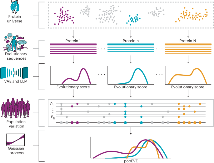
From a methodological perspective, our goal is to rank the severity of genetic variant effects across an individual’s proteome. To achieve this goal, we developed a probabilistic model trained on protein sequence data from both diverse species (UniRef100) and human populations (UKBB or gnomAD). These datasets offer complementary advantages: cross-species sequences reflect millions of years of evolution, revealing conserved patterns linked to structure and function11, while human exome data captures population-specific constraint at the gene level. By combining both, our model aims to accurately predict variant impact across the proteome at single-residue resolution.
In the following sections, we first introduce the models (referred to here as evo models) used for identifying patterns of conservation across diverse organisms. These models provide a ‘fitness’ score for a given sequence of interest by obtaining an estimate for the log odds:
$$\sigma =\log \left(\frac{p({\boldsymbol{x}})}{p({{\boldsymbol{x}}}^{{\rm{ref}}})}\right)\,,$$
(1)
where x represents the sequence of interest and xref is the reference sequence.
We introduce popEVE, a model that predicts the presence or absence of a variant in the human population based on input fitness scores from underlying models. It produces a calibrated score that effectively rescales and ensembles these inputs, enabling comparison of variant effects across different proteins.
Modeling individual proteins using evolutionary data
Recent work has shown that unsupervised models trained on protein sequence distributions across diverse species can distinguish benign from pathogenic variants in known disease genes, performing comparably to functional assays11,64. We use two subtypes of such models: an alignment-based model, which is a variational autoencoder, trained on MSAs of individual genes; and an alignment-free model, inspired by large language models, trained on a full protein database (UniRef90). Below, we summarize each approach.
The Bayesian variational autoencoder (EVE)
Variational autoencoders (VAEs)65,66 are a class of latent variable models that have been shown to be effective at capturing high-dimensional distributions in computer vision67,68, natural language processing69 and more. The assumption underlying a VAE is that the observed high-dimensional distribution is generated by a much smaller number of hidden (also known as latent) variables zi. The generative story is thus:
$$\begin{array}{rcl}{\boldsymbol{z}}& \sim &{\mathcal{N}}(0,{{\boldsymbol{I}}}_{D})\\ p({x}_{i}^{\alpha }| {\boldsymbol{z}},{\boldsymbol{\theta }})&=&{\rm{softmax}}({(\;{f}^{\;{\boldsymbol{\theta }}}({\boldsymbol{z}}))}_{i}^{\alpha })\,,\end{array}$$
(2)
where \({x}_{i}^{\alpha }\) is an indicator function for the presence of amino acid α at position i, and the ‘decoder’ fθ(z) is modeled with a fully connected neural network, with spherical Gaussian prior for the parameters θ. In words, the VAE models the conditional probability of seeing the amino acid α at position i, given the latent variables z. Parameter inference is achieved by the use of amortized inference, where we model the distribution q(z∣xij, θ) with another fully connected neural network, often referred to as the encoder. In previous work11 we found a symmetric relationship between encoder and decoder to work well with three layers, consisting of 2,000–1,000–300 and 300–1,000–2,000 nodes, respectively.
To score a sequence, we use the evidence lower bound (ELBO), which is a lower bound on the log-marginal likelihood p(x):
$$\begin{array}{l}{\rm{ELBO}}({\bf{x}})={N}_{{\rm{eff}}}.{{\mathbb{E}}}_{p({\boldsymbol{x}})}\\\left[{{\mathbb{E}}}_{q({\theta }_{{\bf{p}}}),q({\bf{z}}| {\boldsymbol{x}})}\left(\log p({\boldsymbol{x}}| {\bf{z}},{\theta }_{{\bf{p}}})\right)-{D}_{KL}(q({\bf{z}}| {\boldsymbol{x}},{\phi }_{{\bf{p}}})\parallel p({\bf{z}}))\right]-{D}_{KL}(q({\theta }_{{\bf{p}}})\parallel p({\theta }_{{\bf{p}}}))\end{array}$$
(3)
where \({N}_{{\rm{eff}}}=\mathop{\sum }\nolimits_{n = 1}^{N}{w}_{{x}_{n}}^{{\rm{C}}}\) and \({w}_{{x}_{n}}^{{\rm{C}}}\) is defined in equation (5). The fitness score is then simply
$$\sigma =\log \frac{p({\boldsymbol{x}}| {\theta }_{{\bf{p}}})}{p({{\boldsymbol{x}}}^{{\rm{ref}}}| {\theta }_{{\bf{p}}})}\approx ELBO({\boldsymbol{x}})-ELBO({{\boldsymbol{x}}}^{{\rm{ref}}})$$
(4)
Sequence reweighting
All models used in this work make the false assumption that the training data is independently and identically distributed. This independently and identically distributed assumption breaks down owing to phylogenetic and ascertainment biases. The fact that the VAE is trained on aligned data presents an opportunity to correct for these two biases with sequence reweighting. Following the approach described in previous work70, we re-weight each protein sequence xi from a given MSA according to the reciprocal of the number of sequences in the corresponding MSA within a given Hamming distance cutoff, T.
$${w}_{{{\boldsymbol{x}}}_{n}}^{{\rm{C}}}={\left(\mathop{\sum }\limits_{\begin{array}{c}m = 1\\ m\ne n\end{array}}^{N}{\mathbb{1}}[{\rm{Dist}}({{\boldsymbol{x}}}_{n},{{\boldsymbol{x}}}_{m}) < T\;]\right)}^{-1}$$
(5)
where N is the number of sequences in the MSA, and bold, lowercase x represents a protein sequence, indexed by subscript Latin indices. As in previous work60, we set T = 0.2 for all human proteins.
Masked language model (ESM-1v)
The transformer architecture has enabled the training of single, alignment-free models of essentially all known proteins. In this work, we make use of ESM-1v31, which is trained on UniRef90.
ESM-1v31 is a high-capacity 650 million parameter language model that uses a form of self-supervision known as masking. During training, each sequence has a randomly sampled fraction of its amino acids replaced with a ‘mask’ token, and the network is then trained to predict the amino acids that have been masked. For each masked amino acid, the negative log likelihood of the missing amino acid, conditioned on the sequence context, is independently minimized.
$${\mathcal{L}}={{\mathbb{E}}}_{x \sim X}{{\mathbb{E}}}_{M}\sum _{i\in M}-\log p({x}_{i}| {x}_{/M})\,.$$
(6)
Hence, for the model to successfully perform this task, the dependencies between the masked amino acid and the unmasked sequence context must be learned.
Estimating variant-level constraint in humans using Gaussian processes
The models described above perform well for ranking variants within a given gene but are not effective at comparing variants across genes (Fig. 1 and Supplementary Table 1). This limitation is expected, particularly for alignment-based models, which are trained independently for each coding region. Although several models provide genome-wide scores (for example, Fig. 2e), none have been explicitly designed to rank variant severity across the proteome. To address this gap, we introduced popEVE, the first model aimed at proteome-wide comparison of missense variant effects.
Similar to above, we define the evo score from one of the evo models, which we index A, with \(A\in \left\{1,2\right\}\), as the log odds between the sequence of interest x and some reference sequence xref:
$${\sigma }^{A}=\log \left(\frac{{p}^{A}({\boldsymbol{x}})}{{p}^{A}({{\boldsymbol{x}}}^{{\rm{ref}}})}\right)\,.$$
(7)
In what follows, sequences that differ from the reference sequence by a single amino acid substitution have a special role, so it is convenient to define \({({\sigma }_{i}^{\alpha })}_{n}^{A}\) as the score from model A for a protein sequence, which differs from the reference \({{\boldsymbol{x}}}_{n}^{{\rm{ref}}}\) sequence for protein n solely by having amino acid α at position i.
We expect the probability of observing a sequence in the population to depend, in a fairly simple manner, on the score from the underlying evo models. We adopt a simple Bayesian, non-linear, non-parametric approach to modeling this relationship, with the use of a Bernoulli likelihood and a latent Gaussian process. Specifically, we model the presence or absence of the variant in the UKBB as:
$${p}_{n}^{A}(\;{y}_{i}^{\alpha }| {\sigma }_{in}^{\alpha A})=\,\text{Ber}\,\left({y}_{in}^{\alpha }| \varphi (\;{f}_{n}^{A}({\sigma }_{in}^{\alpha A}))\right)$$
(8)
where \({y}_{ijk}\in \left\{1,0\right\}\) indicates the presence or absence of a variant in the UKBB, the link function φ (⋅) is the inverse logit function (also referred to as the logistic function) \(\varphi (z)=\exp (z){(1+\exp (z))}^{-1}\) and the function \({f}_{n}^{A}(\sigma )\) is drawn from a Gaussian process prior:
$$f(\sigma ) \sim GP(m(\sigma ),{\mathcal{K}}(\sigma ,{\sigma }^{{\prime} })),$$
(9)
with zero mean function m(σ) = 0 and radial basis function kernel
$${\mathcal{K}}(\sigma ,{\sigma }^{{\prime} })=\exp \left(-\gamma {(\sigma -{\sigma }^{{\prime} })}^{2}\right).$$
(10)
The inferred function \({f}_{n}^{A}(\sigma )\) can be thought of as a new fitness score. The intuition is that by modeling the amount of variation seen per protein in the UKBB or gnomAD, \({f}_{n}^{A}(\sigma )\) it essentially rescales the evo score \({\sigma }_{n}^{A}\) to account for the degree of constraint acting on a per-variant basis in the population, and how that constraint depends on \({\sigma }_{n}^{A}\); thus resulting in a score that can rank the pathogenicity of variants across different coding regions.
Efficient function inference by restoring conjugacy with Pólya-gamma data augmentation
For each protein of interest, indexed n, and each underlying evo model, indexed A, we seek to infer the functions \({f}_{n}^{A}\). To do so, we consider the scores of all possible single amino acid substitutions in that protein and their corresponding labels \({y}_{in}^{\alpha }\), indicating if that variant has been observed, or not, in the UKBB (we also provide a version of the model trained on gnomAD instead of the UKBB). Dropping the indices n and A for compactness, we denote the training data as the set of scores \({\boldsymbol{\sigma }}=[{\sigma }_{1}^{1},\ldots ,{\sigma }_{L}^{19}]\in {{\mathbb{R}}}^{N}\) and \({\boldsymbol{y}}=[{y}_{1},\ldots ,{y}_{N}]\in {\left\{0,1\right\}}^{N}\), where L is the number of amino acids in the protein and N = 19L is the total number of possible single amino acid substitutions. Let f = [f1, …, fN] be the function values corresponding to the input σ, then equation (8), together with the Gaussian process prior for f, implies:
$$p(\;{\boldsymbol{f}}| {\boldsymbol{y}},{\boldsymbol{\sigma }})\propto p(\;{\boldsymbol{y}}| {\;\boldsymbol{f}\;})p(\;{\boldsymbol{f}\;}| {\boldsymbol{\sigma }})\,,$$
(11)
where \(p({\boldsymbol{f}}| {\boldsymbol{\sigma }})={\mathcal{N}}({\boldsymbol{f}}| 0,{K}_{NN})\), with KNN denoting the kernel matrix evaluated at the training points. Therefore, in contrast to models with a Gaussian process prior and a Gaussian likelihood, inference is analytically intractable because the Gaussian prior is not conjugate to the Bernoulli likelihood.
One appealing approach to overcoming this issue is to introduce additional latent variables that restore conjugacy. Following previous work71, we introduce the auxiliary variables ω and define the augmented likelihood to factorize as:
$$p(\;{\boldsymbol{y}},{\boldsymbol{\omega }})=p(\;{\boldsymbol{y}}| {\;\boldsymbol{f}},{\boldsymbol{\omega }})p({\boldsymbol{\omega }})$$
(12)
The goal then is to find a prior p(ω) to satisfy two properties: that when marginalizing out ω, the original model is recovered; and the Gaussian prior p(f) is conjugate to the likelihood p(y∣f, ω). These conditions are satisfied by the Pólya-gamma distribution, which may be thought of as an infinite convolution of Gamma distributions; that is, ω ~ PG(b, c), where
$$\omega =\frac{1}{2{\pi }^{2}}\mathop{\sum }\limits_{m=1}^{\infty }\frac{{g}_{m}}{{\left(m-\frac{1}{2}\right)}^{2}+{\left(\frac{c}{2\pi }\right)}^{2}}\,,$$
(13)
and gm ~ Γ(b, 1). Alternatively, we can define the Pólya-gamma distribution in terms of its moment generating function (these two definitions are related by the Laplace transform):
$${{\mathbb{E}}}_{{\rm{PG}}}[\exp (-\omega t)]=\frac{1}{{\cosh }^{b}\left(\sqrt{\frac{t}{2}}\right)}.$$
(14)
This second definition is useful, as it suggests that the logistic link function may be expressed in terms of Pólya-gamma variables
$$\begin{array}{rc}\varphi ({z}_{i})&=\frac{\exp ({z}_{i})}{(1+\exp ({z}_{i}))}\\ &=\frac{\exp\left(\frac{{z}_{i}}{2}\right)}{2\cosh\left(\frac{{z}_{i}}{2}\right)}\\ &=\frac{1}{2}\int\exp \left(\frac{{z}_{i}}{2}-\frac{{z}_{i}^{2}}{2}{\omega }_{i}\right)p({\omega }_{i}){\rm{d}}{\omega }_{i}\,.\end{array}$$
(15)
Hence, substituting zi = yif(σi), we obtain
$$p(\;{\boldsymbol{y}}| {\boldsymbol{\omega }},{\boldsymbol{f}\;})\propto \exp \left(\frac{1}{2}{{\boldsymbol{y}}}^{\top }{\boldsymbol{f}}-\frac{1}{2}{{\boldsymbol{f}}}^{\top }\Omega {\boldsymbol{f}}\right)\,,$$
(16)
where Ω = diag(ω) is the diagonal matrix of the Pólya-gamma variables. This augmented likelihood is conjugate to p(f) as required.
Developed in prior work72, once conditional conjugacy is restored, it is possible to derive closed-form updates for variational inference with natural gradients and a learning rate close to one, enabling highly efficient inference of f.
Making the models scale with inducing points
Inference in GPs with a Gaussian likelihood, while exact, take \({\mathcal{O}}({N}^{3})\) time, and hence additional methods are required to perform inference when the training data are large. One such method is to learn a ‘summary’ of the data with M ≪ N pseudo inputs, otherwise known as inducing points73, and hence reduce the complexity to \({\mathcal{O}}({M}^{3})\). Following the prior work72, we introduce M additional variables u = [u1, …, uM], where the function values of the GP f are related to u by
$$\begin{array}{lc}p(\;{\boldsymbol{f}}| {\boldsymbol{u}})={\mathcal{N}}(\;{\boldsymbol{f}\;}| {K}_{NM}{K}_{MM}^{-1}{\boldsymbol{u}},\tilde{K})\\ p({\boldsymbol{u}})={\mathcal{N}}({\boldsymbol{u}}| 0,{K}_{MM})\,,\end{array}$$
(17)
where kMM is the kernel matrix resulting from evaluating the kernel at the M inducing points, KNM is the kernel between the training points and the inducing points and \(\tilde{K}={K}_{NN}-{K}_{NM}{K}_{MM}^{-1}{K}_{MN}\).
Hence, the complete joint distribution of our model is given by
$$p(\;{\boldsymbol{y}},{\boldsymbol{\omega }},{\boldsymbol{f}},{\boldsymbol{u}})=p(\;{\boldsymbol{y}}| {\boldsymbol{\omega }},{\boldsymbol{f}\;})p({\boldsymbol{\omega }})p(\;{\boldsymbol{f}\;}| {\boldsymbol{u}})p({\boldsymbol{u}})\,.$$
(18)
Implementation
This model is implemented in GPyTorch74 and is publicly available through a dedicated GitHub repository.
Ensembles of models with only partially intersecting domains
Ensembles of models can often achieve a performance similar to, and sometimes even stronger than, the strongest constituent model75. Our setup provides a novel opportunity to build a highly performant ensemble model by incorporating the scores from multiple evo models. By training a separate Gaussian process model for each evo model, we naturally create directly comparable scores between models, thereby enabling the typical, but potentially problematic, standardization step to be bypassed entirely. We define the popEVE score \(\bar{\sigma }\) to simply be the mean of the means of the posteriors of each GP, for each evo model whose domain contains the variant of interest.
$${\bar{\sigma }}_{ij}^{{\rm{\alpha }}}=\frac{1}{{Q}_{ij}^{A}}\mathop{\sum }\limits_{A=1}^{{Q}_{ij}^{\alpha }}{\mathbb{E}}\left[{f}_{j}^{A}({\sigma }_{i}^{\alpha })\right]\,,$$
(19)
where \({Q}_{ij}^{A}\) is the number of evo models capable of making a prediction for the amino acid substitution α at position i in protein j.
Performance assessments
We evaluated key properties of our model with a number of clinically relevant tasks and compared its performance with pre-existing models, whose scores were downloaded from dbNSFP (v.4.7)76 (we use the same set of models that were analyzed in a previous publication23).
Comparing model performance within proteins
To assess model performance at ranking the pathogenicity of variants within the same gene, similar to prior work11, we consider two tests: correlation of model predictions with deep mutational scans and ability to predict benign and pathogenic labels in ClinVar.
To assess concordance with deep mutational scans, we compute the Spearman’s correlation between the model score and reported experimental fitness (for example, expression) (Extended Data Fig. 2). To assess the ability to separate benign from pathogenic variants, we made use of two curated sets of ClinVar labels as described in ‘ClinVar benign and pathogenic variants’. We computed the area under the receiver operating characteristic curve for all genes with at least five benign and five pathogenic labels. With these sets, we were able to assess the performance across 50 and 31 proteins and in 2019 and 2020 datasets, respectively (Extended Data Fig. 1).
Comparing model performance across proteins
Ranking clinical pathogenic variants by severity
To evaluate how well models rank clinical pathogenic variants by severity, we assembled a set of ClinVar 1+ star variants linked to phenotypes with childhood or adult onset or death, based on OrphaNet annotations35. For each model, we identified the 5th percentile score threshold for benign ClinVar variants and used this as a reference. We then compared the log odds of childhood-versus-adult-associated pathogenic variants falling below this threshold. Pairwise z-scores and P values were computed to assess whether model differences were statistically significant. Models focused solely on pathogenicity are expected to perform poorly, whereas those capturing variant fitness and phenotypic severity should distinguish between childhood and adult onset variants.
Distinguishing SDD cases from unaffected controls
We next evaluated the model’s ability to rank variant severity across the proteome and across individuals. To do so, we constructed a test set from de novo variants found in patients with SDDs and unaffected siblings of individuals with autism spectrum disorder. The goal was to determine whether the model could distinguish cases carrying likely pathogenic de novo variants from controls with variants not expected to contribute to disease.
We defined ‘cases’ as individuals with at least one de novo variant in a known DD gene (DDG2P, downloaded January 2023), following the approach of a previous publication8. However, only a subset of these variants is expected to be truly pathogenic. Based on an observed excess of 2,982 de novo missense variants among 5,625 cases, we estimate that approximately 53% carry a causal variant. Accordingly, we adjusted the maximum achievable recall to reflect this expected upper bound.
This test set (Supplementary Table 5) allows us to benchmark model performance in a realistic clinical setting. popEVE outperforms all current state-of-the-art models for pathogenicity prediction, including the underlying evolutionary models it builds upon (Fig. 3b, Extended Data Fig. 9a and Supplementary Table 1).
Assessing overprediction of deleterious variants in the general population
We evaluated each model’s ability to recover SDD cases from de novo mutations or WES while minimizing false positives in the general population. For each model and score threshold, we computed the percentage of individuals in the UKBB and SDD metacohort (or DDD sub-cohort) with at least one variant as or more pathogenic (Fig. 2h,k and Supplementary Fig. 10d,f), comparing the cumulative distributions between cases and controls. For the SDD metacohort, we used individuals with de novo missense variants in genes previously implicated by DeNovoWEST8, representing high-confidence diagnoses.
To assess prioritization of causal variants, we calculated the fraction of DDD individuals whose de novo variant was ranked more pathogenic than all inherited variants at each threshold. At −5.056, 513 individuals had a qualifying variant, and in 98% of cases, it ranked as the most deleterious. The rate of decay reflects each model’s genome-wide ranking ability.
Analysis of patient data
We explored two approaches to analyzing de novo mutations from a metacohort composed of subjects from the DDD study, GeneDx and Radboud Medical Center in the hope that popEVE may provide novel evidence for the genetic diagnosis of currently unsolved cases: burden testing of variants per gene across the full cohort, and per-patient direct case–variant association.
Direct case–variant association
Based on the set of de novo variants from cases and controls, we constructed a Bayesian Gaussian mixture model to determine a score cutoff as:
$$\begin{array}{rcl}{{\mathbf{\mu }}}_{1}& \sim &{\mathcal{N}}({{\mathbf{\mu }}}_{0},{{\mathbf{\Sigma }}}_{0})\\ {{\mathbf{\mu }}}_{2}& \sim &{\mathcal{N}}({{\mathbf{\mu }}}_{0},{{\mathbf{\Sigma }}}_{0})\\ {\lambda }_{1}& \sim &\,\text{Lognormal}\,({\mu }_{\lambda },{\sigma }_{\lambda })\\ {\lambda }_{2}& \sim &\,\text{Lognormal}\,({\mu }_{\lambda },{\sigma }_{\lambda })\\ {\mathbf{\pi }}& \sim &\,\text{Dirichlet}\,({\mathbf{\alpha }})\\ \,\text{For}\,i=1,\ldots ,N:\\ \hspace{0.5em}{a}_{i}& \sim &\,\text{Categorical}\,({\mathbf{\pi }})\\ \hspace{0.5em}{{\bf{x}}}_{i}& \sim &{\mathcal{N}}({{\mathbf{\mu }}}_{{a}_{i}},{\lambda }_{{a}_{i}})\end{array}$$
(20)
where μ0 = −3.6 and Σ0 = 0.7. We then identified an uncertainty cutoff corresponding to a greater than 99.99% likelihood of being in the lower fitness distribution, \(\bar{\sigma }\le -5.056\). We found that constructing the model with solely the de novo variants from the cases resulted in a similar threshold.
Using the threshold \(\bar{\sigma }\le -5.056\), we searched the full DD cohort for individuals with at least one de novo missense variant below this score and no predicted LoF variants. For these individuals, we consider the identified missense variant a strong candidate for being causal. In addition to the high accuracy of the Gaussian mixture model, these variants show strong enrichment relative to the background mutation rate (Fig. 3d), further supporting their likely pathogenicity.
Gene-collapsing model
To compare with previous methods, we implemented gene-collapsing models for the SDD cohort following the DeNovoWEST framework8. For each gene, we estimated the probability of observing a total score ≥xobs by testing mutation counts (0 to N) until the Poisson likelihood, based on expected de novo mutation rates, fell near zero. Context-dependent mutation rates from Samocha et al. (2014)29 were used to estimate expected counts and sample variants. We ran 10,000 simulations per gene. To adjust for multiple testing, we also assessed the likelihood of observing a score ≥xobs anywhere in the proteome.
$$p(\,\text{gene}\,)=\mathop{\sum }\limits_{n=0}^{N}P(n={n}_{gene}| {\lambda }_{gene})P({x}_{gene}\le {x}_{obs}| n)P({x}_{proteome}\le {x}_{obs}| n)$$
(21)
We selected our significance cutoff by dividing 0.05 by the total number of tests (or total number of genes or proteins we have modeled): p < 0.05 / 18,395. We also performed gene collapsing on the unaffected controls using the same method.
Structural and functional analysis of deleterious mutationsFunctional similarity of novel and known DD genes
We compared the functional properties of our novel genes with comparison to known DD genes37 across features known to differentiate DD genes from genes not associated with DDs, similar to previous work8. We calculated the enrichment of these variables in either our novel genes or known DD genes compared to non-DD genes (Fig. 6d, Extended Data Fig. 8 and Supplementary Tables 8 and 9).
For interactions, we selected protein–protein interactions (BioGRID77) enriched in known DD genes compared to non-DD genes. To ensure that these interactions are generalizable, we selected those that are significantly enriched in known DD genes (P < 0.05 after Benjamini–Hochberg correction) and present in at least 10% of known DD genes (n > 223). Median expression, measured in reads per kilobase of transcript per million mapped reads, in the fetal brain was determined across samples from the Allen Brain Atlas78. For the relevant Gene Ontology terms Molecular Function and Biological Processes, we selected terms enriched in known DD genes compared to non-DD genes using DAVID79. To ensure these terms are generalizable, we selected those that are significantly enriched in known DD genes (P < 0.05 after Benjamini–Hochberg correction) and present in at least 10% of known DD genes (n > 223). Haploinsufficient is a binary variable of genes with evidence of haploinsufficiency (dosage pathogenicity level three) from the ClinGen Dosage Sensitivity Map55; human essential is a binary variable of whether a gene was deemed essential in human cell lines based on CRISPR screens53; ACMG genes is a binary variable indicating whether a gene is a clinically actionable gene according to the American College of Medical Genetics and Genomics (v.2.0)80; somatic drivers is a binary variable of whether the gene is known to be a somatic driver gene81; mouse essential is a binary variable of whether a gene is essential in mice; that is, homozygous knockouts of that gene resulted in lethality52,82; and LoF tolerant is a binary variable of whether a gene is tolerant of homozygous LoF mutations in humans18.
Functional network
We created a functional gene network with 123 de novo novel genes from popEVE (with a 99.99 threshold) and significant genes from DeNovoWEST8 using STRING83, as shown in Extended Data Fig. 9a and Supplementary Table 10. We show edges from medium-confidence (0.4) experiments. Genes were denoted as previously discovered if they were already observed in DDG2P37 or DeNovoWEST.
Additionally, we used medium-confidence (0.4) experiment annotations to calculate the average node degree of DDG2P genes and DeNovoWEST genes with and without our significant popEVE genes included, both from de novo analysis and no-trios analysis (Extended Data Fig. 9b). To determine the relative difference that the significant genes make versus a random set of genes, we performed t-tests 100,000 times with random samples of genes from the whole human genome (with the known and popEVE genes excluded).
Manual structure analysis
From the 131 novel popEVE mutations, we individually investigated structures for the top 20 most predicted deleterious. We only analyzed cryo-electron microscopy or crystallographic structures where our mutation is included in the resolved protein structure. To enhance our analysis, we prioritized structures that exhibited interactions with other proteins and/or ligands. This allowed us to capture and understand the potential consequences of these interactions. All distances listed were calculated with the distance function in PyMol.
Comparative analysis of protein–ligand interactions using a null model
We compared de novo variants from the SDD metacohort and inherited variants from the DDD subset against a null model, which calculated the distance from each position on the variant-containing chain to the nearest ligand. Resolved crystal structures were processed using the Evcouplings PDB reader, with distances computed using the Evcouplings compare package61. Z-scores were computed by subtracting the mean chain-wide distance (excluding the variant site) from the variant-to-ligand distance. Variants were excluded if the chain length differed from the full protein length by more than two standard deviations. Full results are in Supplementary Table 11.
Functional interactions in 3D structures for high-scoring pathogenic variants
3D structures of proteins with high-scoring pathogenic variants were retrieved by alignment to SIFTS database sequences84 using EVcouplings61 with one HMMER iteration62 and a 0.2 bits per residue threshold. A variant was considered to have evidence of functional interaction if, in any matched structure, its position contacted a non-self PDB entity within 8 Å, excluding water and common crystallographic additives (entity info from PDBe REST API40).
Reporting summary
Further information on research design is available in the Nature Portfolio Reporting Summary linked to this article.